10 R Session 04
Stochastic SIR models

review of basic algorithms for stochastic epidemic models
This session is under active development and is subject to change.
10.1 Setup
This R-session will go in parallel with the lecture on stochastic algorithms. First we’ll go through the basics of each algorithm in the lecture and then we’ll walk through the code and you can implement it for yourselves.
10.2 What is stochasticity and where does it come from?
Much of the world is uncertain (i.e. we don’t know exactly how things work, what values are, or what tomorrow will hold). Some of that uncertainty is, at least theoretically, knowable and some is not. For example, in our discussion of estimating \(R_0\), there may be a very real \(R_0\) for a given population and pathogen, even if we don’t know it. Thus, our estimate of \(R_0\) may be “uncertain” (e.g. has a confidence interval around it, reflecting our certainty), but the models we’ve been developing so far are “deterministic”, so conditional on a given value of \(R_0\) the resulting epidemic curve is exactly specified by the model. If we return to the code from R-session 1, we can plot a single deterministic realization of a model with \(R_0 = 1.8\).
Code
sir_model <- function(time, state, params, ...) {
  transmission <- params["transmission"]
  recovery <- 1 / params["duration"]

  S <- state["S"]
  I <- state["I"]
  R <- state["R"]

  dSdt <- -transmission * S * I
  dIdt <- (transmission * S * I) - (recovery * I)
  dRdt <- recovery * I

  return(list(c(dSdt, dIdt, dRdt)))
}
Code
# Turn the output from the ODE solver into a tibble (dataframe)
# so we can manipulate and plot it easily
sir_sol_df <- as_tibble(sir_sol) %>%
  # Convert all columns to numeric (they are currently type
  # deSolve so will produce warnings when plotting etc)
  mutate(
    # Rather than repeatedly type the same function for every
    # column, use the across() function to apply the function
    # to a selection of columns
    across(
      # The cols argument takes a selection of columns to apply
      # a function to. Here, we want to apply the as.numeric()
      # function to all columns, so we use the function
      # everything() to select all columns.
      .cols = everything(),
      .fns = as.numeric
    )
  ) %>%
  # Convert the dataframe from wide to long format, so we have a
  # column for the time, a column for the state, and a column
  # for the proportion of the population in that state at that
  # time
  pivot_longer(
    # Don't pivot the time column
    cols = -time,
    names_to = "state",
    values_to = "proportion"
  ) %>%
  # Update the state column to be a factor, so the plot will
  # show the states in the correct order
  mutate(state = factor(state, levels = c("S", "I", "R")))

sir_colors <- c(S = "#1f77b4", I = "#ff7f0e", R = "#FF3851")

ggplot(sir_sol_df, aes(x = time, y = proportion, color = state)) +
  geom_line(linewidth = 1.5) +
  scale_color_manual(values = sir_colors) +
  labs(
    x = "Time",
    y = "Fraction",
    color = "State"
  ) +
  theme(legend.position = "top")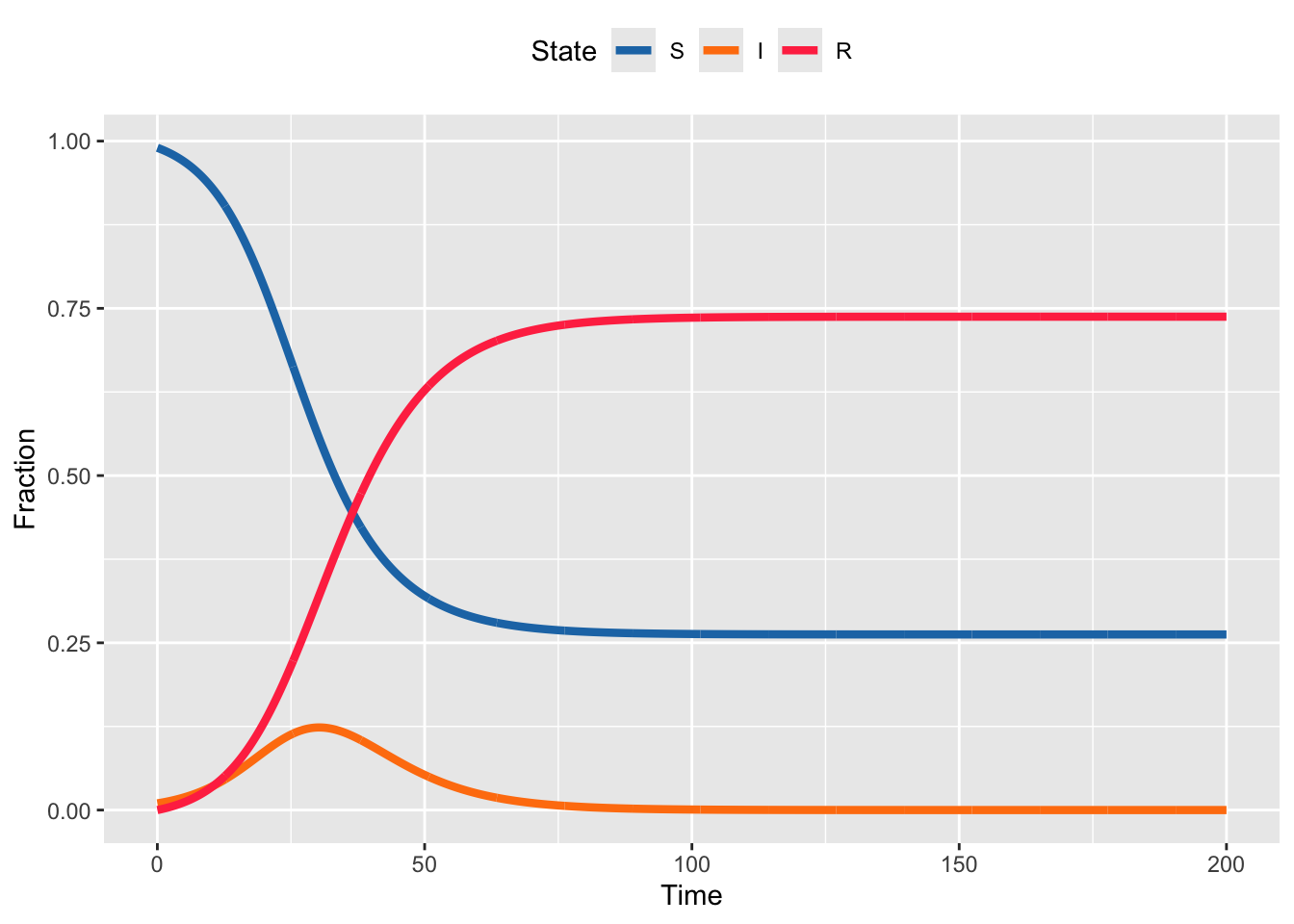
Now, perhaps we used the tools from R-session 3 to estimate \(R_0\) and we think a reasonable \(95\%\) confidence interval for \(R_0\) is \((1.7,1.9)\). If we’re quite certain the duration of infection is 6 days, then that means our corresponding confidence interval on the transmission rate is \((.283,.317)\). An entirely reasonable way to represent this uncertainty in the estimate of the transmission rate is to generate many random draws from within the confidence interval for the transmission rate and examine the resulting epidemic curves. For this we can modify the code above with a loop that does this multiple times.
Code
# the number of times we want to do this.
# This is a matter of choice and computational capacity
# (this model is small and quick, but that won't always be the case)
num_iterations <- 100

# since we're going to do this num_iterations times we need a place
# to store the results

for (iter in 1:num_iterations) {
  # each time take a random draw of the transmission rate from the
  # confidence interval
  sir_params <- c(transmission = runif(1, .283, .317), duration = 6)
  sir_init_states <- c(S = 0.99, I = 0.01, R = 0)
  sim_times <- seq(0, 200, by = 0.1)

  sir_sol <- ode(
    y = sir_init_states,
    times = sim_times,
    func = sir_model,
    parms = sir_params
  )
  sir_sol <- as_tibble(sir_sol)
  # mark this as the iter iteration of the loop
  sir_sol$iteration <- iter
  # if this is the first iteration, create a place to store the output
  # if it's the second or higher, append the output to the storage
  if (iter == 1) {
    sir_sol_storage <- sir_sol
  }
  if (iter > 1) {
    sir_sol_storage <- rbind(sir_sol_storage, sir_sol)
  }
}
Code
# Turn the output from the ODE solver into a tibble (dataframe)
# so we can manipulate and plot it easily
sir_sol_df <- as_tibble(sir_sol_storage) %>%
  # Convert all columns to numeric (they are currently type deSolve
  # so will produce warnings when plotting etc)
  mutate(
    # Rather than repeatedly type the same function for every column,
    # use the across() function to apply the function to a selection
    # of columns
    across(
      # The cols argument takes a selection of columns to apply
      # a function to. Here, we want to apply the as.numeric()
      # function to all columns, so we use the function
      # everything() to select all columns.
      .cols = everything(),
      .fns = as.numeric
    )
  ) %>%
  # Convert the dataframe from wide to long format, so we have a
  # column for the time, a column for the state, and a column
  # for the proportion of the population in that state at that
  # time
  pivot_longer(
    # Don't pivot the time column
    cols = -c(time, iteration),
    names_to = "state",
    values_to = "proportion"
  ) %>%
  # Update the state column to be a factor, so the plot will
  # show the states in the correct order
  mutate(state = factor(state, levels = c("S", "I", "R")))

sir_colors <- c(S = "#1f77b4", I = "#ff7f0e", R = "#FF3851")

ggplot(
  sir_sol_df,
  aes(
    x = time,
    y = proportion,
    color = state,
    group = interaction(iteration, state)
  )
) +
  geom_line(linewidth = 1.5, alpha = .1) +
  scale_color_manual(values = sir_colors) +
  labs(
    x = "Time",
    y = "Fraction",
    color = "State"
  ) +
  guides(color = guide_legend(override.aes = list(alpha = 1))) +
  theme(legend.position = "top")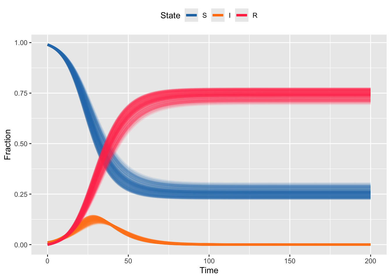
Here note that we are still using our original code for the SIR model, so first we randomly draw the transmission rate, then conditional on that value, we run the deterministic model. Note that each run of the model still has the smooth curves, but each draw is a different set of smooth curves.
There are lots of ways you could extend this. Note that since we are drawing the transmission rate and fixing the duration of infection, the \(R_0\) is slightly different in each simulation. You could make each run have the same \(R_0\) by recalculating the duration of infection based on the random draw of transmission rate; e.g. \(R_0=1.8 = 0.29 * L\) means that \(L=5.5\), so to ensure \(R_0\) is the same in each run, you would need to change \(L\) for each random draw. Alternatively, you might have uncertainty about transmission and duration, so could for e.g. make random draws for both (which would again give a setting where \(R_0\) varies from run to run). None of these are more correct than another, the use case depends on which elements \(R_0\), transmission, duration of infection, you are uncertain about.
In each of the above, the model is , meaning that for a given set of parameters, the resulting outbreak trajectory is always the same. For a model, each run of the model will vary, even if the parameters are the same. This is because each event that occurs (e.g. someone getting infected or recovering) is analogous to a coin flip; even though the rules of the coin (the parameters) are always the same, the side it lands on is random. Unlike a deterministic model, to fully understand the behavior of a stochastic model, you need to run it more than one time, often many times, so these are necessarily more time consuming to work with.
There are many, many ways to make stochastic models and the steps can be way more complicated than flipping coins. But there some foundational versions of these models that illustrate the trade-offs between exact representations of the random processes we think are happening and the computational time it takes to generate outputs. For what we’ll do here, everything will be kind of fast, but in practice, for models of realistic scale, even a single stochastic run can take a while. And if you have to do thousands of runs, even shaving a few seconds or minutes can be important.
10.3 The Gillespie Algorithm
The Gillespie algorithm is the most explicit translation of the ODE form of the SIR model into a stochastic model. It achieves this by noting that ODE-based models are written in terms of the rates at which events occur. At any given point in time, the rate of all events in the ODE is known; what known, is which of the possible events will happen first. Note that even though we expect that the next thing to happen will be the thing that happens with the highest rate, it’s possible that another thing may happen first by random chance. And then, since the rates in the SIR model are dependent on the value of the states (e.g. new infections depend on \(\beta\) and S and I) any change in the states then changes the rates and the likelihood of what will happen next.
The Gillespie algorithm proceeds by 1) calculating all the current rates, 2) randomly drawing exponential random variables that equate to the time until each event happens (recall we talked about the relationship between rate and time in the lectures), then 3) comparing those times and assuming that the next event to occur is the one that had the smallest randomly drawn time. Then you increment the states; e.g. an infection increases I by 1, reduces S by 1, and doesn’t change R. Importantly, you then increment time forward by a step equal to the time until first event occurred. Then you recalculate the rates and randomly draw times, etc, and keep doing this over and over again. For this SIR model, that keeps happening until you run out of infected individuals and there are no new events that can happen.
Code
####################################################################
# Parameters and initial conditions                                #
####################################################################

S <- 998 # number susceptible
I <- 1 # number infected
R <- 1 # number recovered
time <- 0

beta <- 0.5 # transmission rate
gamma <- 1 / 7 # recovery rate
Code
####################################################################
# Gillespie Step                                                   #
####################################################################
gil_step <- function(SIR, beta, gamma) {
  # SIR is a vector containing 4 elements
  #   S = scalar number of susceptibles now
  #   I = scalar number of infecteds now
  #   R = scalar number of recovereds now
  #   time = current time
  # beta = transmission rate
  # gamma = recovery rate

  # draw two random exponential variables
  times <- rexp(
    2,
    c(
      # the first is the rate of new infections: S*Beta*I/N
      beta * SIR[1] * SIR[2] / sum(SIR[1:3]),
      # the second is the rate of new recoveries: I*gamma
      SIR[2] * gamma
    )
  )

  return(list(
    # which.min identifies which of the two random variables is smallest,
    # and thus the first to happen: this is the transition that we'll make
    change_state = which.min(times),
    # this identifies how much time elapsed before the transition occurred,
    # so we can increment time forward
    time_step = min(times)
  ))
}
The gil_step() function increments the states forward by 1 event. Which event happens first, and the time it takes for that event to happen are both random variables. We then need to do this many times.
Code
####################################################################
# Simulate over time                                               #
####################################################################
# here we set the random seed. This isn't necessary in general, but it allows us to write a "random" simulation
set.seed(101)
counter <- 0 # set counter at 0
while (all(I > 0)) {
  # continue until I is depleted
  counter <- counter + 1
  # counter for number of transitions: we don't know how many transitions
  # will happen until the simulation is over
  #
  # current SIR states
  sir_tmp <- c(S[counter], I[counter], R[counter], time[counter])
  step <- gil_step(sir_tmp, beta, gamma)
  if (step$change_state == 1) {
    # if transition is an infection, reduce S and increase I
    sir_tmp[1] <- sir_tmp[1] - 1
    sir_tmp[2] <- sir_tmp[2] + 1
  }
  if (step$change_state == 2) {
    # if transition is an recovery, reduce I and increase R
    sir_tmp[2] <- sir_tmp[2] - 1
    sir_tmp[3] <- sir_tmp[3] + 1
  }
  sir_tmp[4] <- sir_tmp[4] + step$time_step # increment time

  # Append changes
  S <- c(S, sir_tmp[1])
  I <- c(I, sir_tmp[2])
  R <- c(R, sir_tmp[3])
  time <- c(time, sir_tmp[4])

  # cat(S[counter],\"-\",I[counter],\"-\",R[counter],\"-\",time[counter], \".\\n\")
  # this prints the output as it goes
  # reset the seed so that every subsequent simulation IS random
  set.seed(NULL)
}
We can now plot the one realization of this stochastic outbreak. Notice that it has the same general shape as the deterministic outbreak, but is no longer smooth because each individual event over time happens randomly.
Code
# Reuse the plotting code from above

# Turn the output from gil_step() into a tibble (dataframe)
# so we can manipulate and plot it easily
# put elements in a data frame
gil_df <- tibble(time, S, I, R) %>%
  # Convert all columns to numeric (they are currently type
  # deSolve so will produce warnings when plotting etc)
  mutate(
    # Rather than repeatedly type the same function for every
    # column, use the across() function to apply the function
    # to a selection of columns
    across(
      # The cols argument takes a selection of columns to apply
      # a function to. Here, we want to apply the as.numeric()
      # function to all columns, so we use the function
      # everything() to select all columns.
      .cols = everything(),
      .fns = as.numeric
    )
  ) %>%
  # Convert the dataframe from wide to long format, so we have a
  # column for the time, a column for the state, and a column
  # for the proportion of the population in that state at that
  # time
  pivot_longer(
    # Don't pivot the time column
    cols = -c(time),
    names_to = "state",
    values_to = "number"
  ) %>%
  # Update the state column to be a factor, so the plot will
  # show the states in the correct order
  mutate(state = factor(state, levels = c("S", "I", "R")))

sir_colors <- c(S = "#1f77b4", I = "#ff7f0e", R = "#FF3851")

ggplot(gil_df, aes(x = time, y = number, color = state)) +
  geom_line(linewidth = 1.5) +
  scale_color_manual(values = sir_colors) +
  labs(
    x = "Time",
    y = "Number",
    color = "State"
  ) +
  theme(legend.position = "top")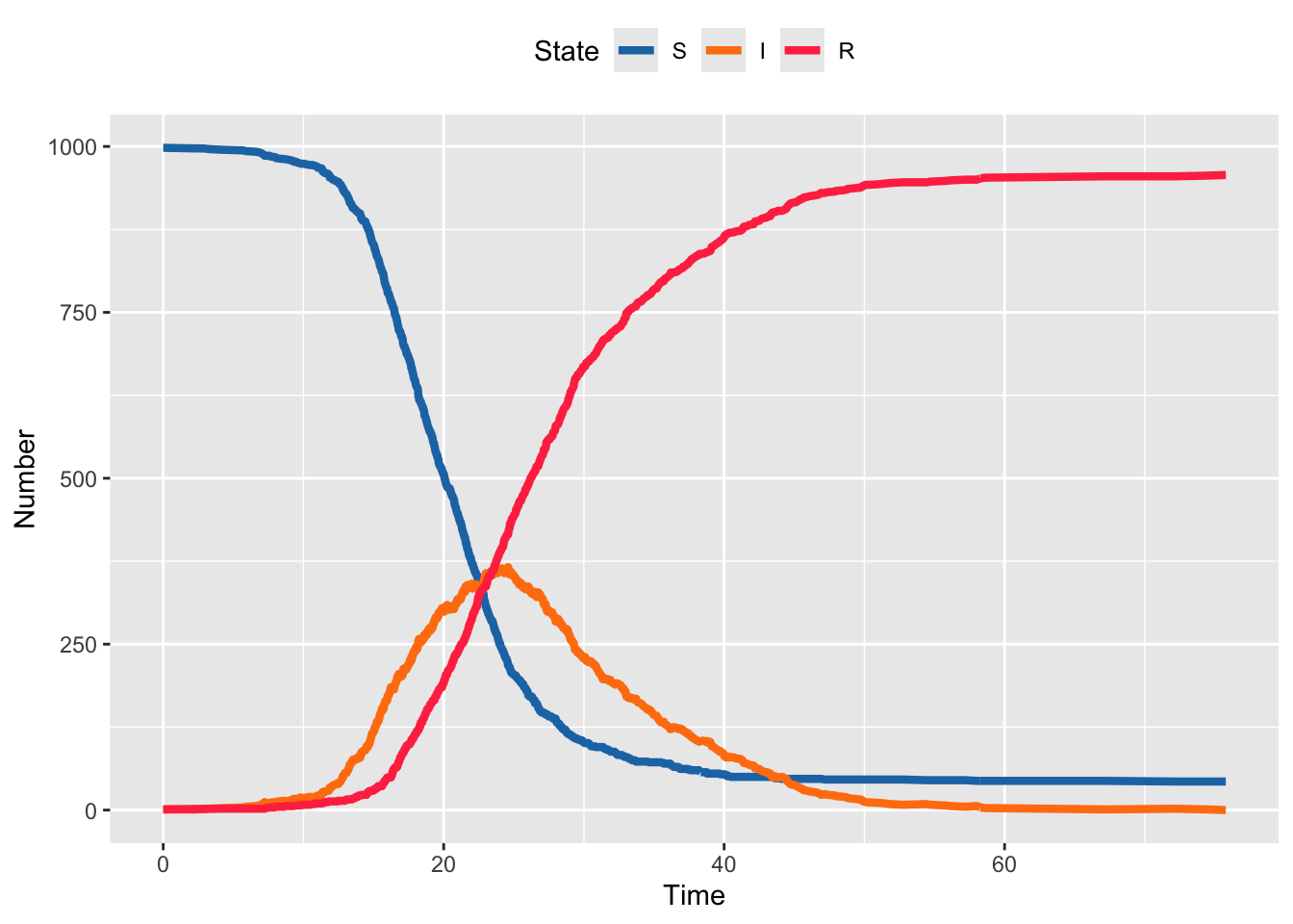
Because each realization is stochastic, we need to generate many runs to see the general behavior. The code below runs 10 iterations. Generally, this would be considered a very small number of iterations. But even for this very small model, running 100 or more means you’ll be waiting for output. Note that this code is designed to be transparent not to be fast. Making these run fast is beyond the scope of this assignment.
Code
####################################################################
# Simulate over time                                               #
num_iterations <- 10 # number of realizations to simulate

for (iter in 1:num_iterations) {
  ####################################################################
  # Parameters and initial conditions                                #
  ####################################################################

  S <- 998 # number susceptible
  I <- 1 # number infected
  R <- 1 # number recovered
  time <- 0
  # initialize iteration counter
  iteration <- iter

  beta <- .5 # transmission rate
  gamma <- 1 / 7 # recovery rate

  ####################################################################
  # Simulate over time                                               #
  ####################################################################
  counter <- 0 # set counter at 0
  while (all(I > 0)) {
    # continue until I is depleted
    counter <- counter + 1
    # counter for number of transitions: we don't know how many transitions
    # will happen until the simulation is over

    # current SIR states
    sir_tmp <- c(S[counter], I[counter], R[counter], time[counter])
    step <- gil_step(sir_tmp, beta, gamma)
    if (step$change_state == 1) {
      # if transition is an infection, reduce S and increase I
      sir_tmp[1] <- sir_tmp[1] - 1
      sir_tmp[2] <- sir_tmp[2] + 1
    }
    if (step$change_state == 2) {
      # if transition is an recovery, reduce I and increase R
      sir_tmp[2] <- sir_tmp[2] - 1
      sir_tmp[3] <- sir_tmp[3] + 1
    }
    # increment time
    sir_tmp[4] <- sir_tmp[4] + step$time_step

    # Append changes
    S <- c(S, sir_tmp[1])
    I <- c(I, sir_tmp[2])
    R <- c(R, sir_tmp[3])
    time <- c(time, sir_tmp[4])
    iteration <- c(iteration, iter)

    # cat(S[counter],\"-\",I[counter],\"-\",R[counter],\"-\",time[counter], \".\\n\")
    # this prints the output as it goes
  }
  if (iter == 1) {
    sir_gil_storage <- tibble(S, I, R, time, iteration)
  }
  if (iter > 1) {
    sir_gil_storage <- bind_rows(
      sir_gil_storage,
      tibble(S, I, R, time, iteration)
    )
  }
}
Code
# Reuse the plotting code from above

# Turn the output from gil_step() into a tibble (dataframe)
# so we can manipulate and plot it easily
# put elements in a data frame
gil_df <- sir_gil_storage %>%
  # Convert all columns to numeric (they are currently type
  # deSolve so will produce warnings when plotting etc)
  mutate(
    # Rather than repeatedly type the same function for every
    # column, use the across() function to apply the function
    # to a selection of columns
    across(
      # The cols argument takes a selection of columns to apply
      # a function to. Here, we want to apply the as.numeric()
      # function to all columns, so we use the function
      # everything() to select all columns.
      .cols = everything(),
      .fns = as.numeric
    )
  ) %>%
  # Convert the dataframe from wide to long format, so we have a
  # column for the time, a column for the state, and a column
  # for the proportion of the population in that state at that
  # time
  pivot_longer(
    # Don't pivot the time column
    cols = -c(time, iteration),
    names_to = "state",
    values_to = "number"
  ) %>%
  # Update the state column to be a factor, so the plot will
  # show the states in the correct order
  mutate(state = factor(state, levels = c("S", "I", "R")))

sir_colors <- c(S = "#1f77b4", I = "#ff7f0e", R = "#FF3851")

ggplot(
  gil_df,
  aes(
    x = time,
    y = number,
    color = state,
    group = interaction(iteration, state)
  )
) +
  geom_line(linewidth = 1.5, alpha = .1) +
  scale_color_manual(values = sir_colors) +
  labs(
    x = "Time",
    y = "Number",
    color = "State"
  ) +
  guides(color = guide_legend(override.aes = list(alpha = 1))) +
  theme(legend.position = "top")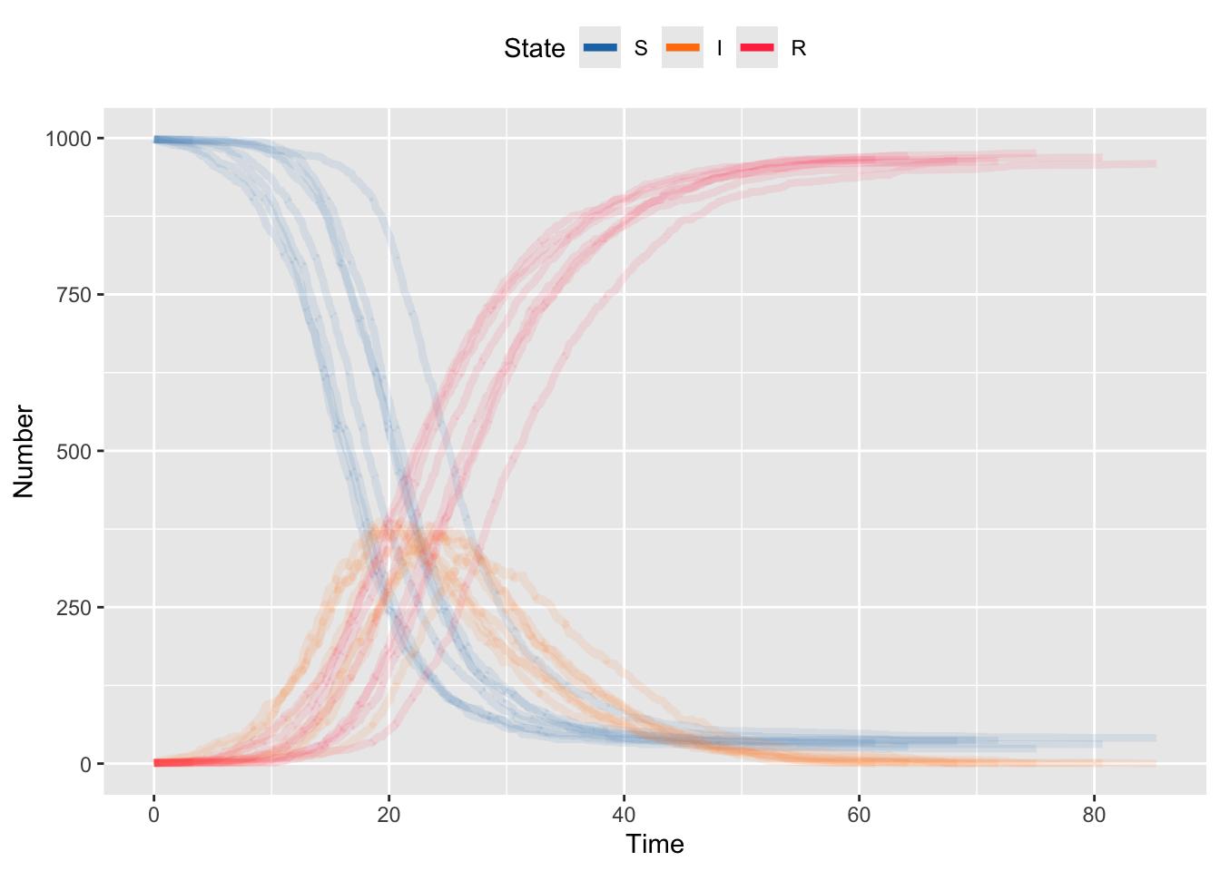
The Gillespie algorithm doesn’t cut any corners relative to the ODE model, but that comes at the cost of computational efficiency. For every event that happens (e.g. an infection) you also have to generate a random draw (e.g. a recovery) that you don’t use, except for comparison. And the bigger your population, the more possible events can happen. So the bigger the model (e.g. adding exposed or vaccinated classes, or heterogeneity, add transitions) and the bigger the population, the more calculation you need and and therefore the slower the model.
10.4 The Tau Leaping Algorithm
The Gillespie algorithm is great because it is an exact interpretation of the transitions in the ODE model: every change of state (e.g. infection or recovery) changes the rates for the next transition. Doing this comes at a computational cost. One reasonable approximation is the Tau Leaping algorithm. Here, we move in discrete chunks of time and make random draws for multiple events occurring within that chunk. Here the computation scales with the number of time steps (and the number of states requiring transitions). But, we rely on the result that, if rates stay constant, the number of events that occur in a discrete chunk of time can be approximated by a Poisson random variable. Thus, we don’t need to make random draws for every event. Instead we can make 1 draw for the multiple events that will occur in 1 day, or 1 week, etc. The key here is the assumption that the rates stay constant; since each new infection or recovery will change the rates, we don’t want to occur (in which case the rate at the start of the time step will be very different than the rate at the end of the time step). So we are faced with a trade-off; very small time steps don’t violate the assumptions, but the smaller the steps, the closer we are to Gillespie and the smaller the computational savings. There’s no right answer to what time step to use. Here we’ll use 1 day, for convenience.
Code
####################################################################
# Parameters and initial conditions                                #
####################################################################

S <- 998 # number susceptible
I <- 1 # number infected
R <- 1 # number recovered
time <- 0

beta <- .5 # transmission rate
gamma <- 1 / 7 # recovery rate
Code
####################################################################
# Tau Leaping Single time step                                     #
####################################################################
tau_sir_step <- function(sims, S, I, R, beta, gamma, delta_t, ...) {
  # adapted from Aaron King's code
  # sims = number of simulations
  # S = initial susceptible population
  # I = initial infected population
  # R = initial recovered population
  # beta = transmission rate
  # gamma = recovery rate

  # total population size
  N <- S + I + R
  # new incident infections
  dSI <- rpois(n = sims, beta * S * (I / N) * delta_t)
  # recoveries
  dIR <- rpois(n = sims, gamma * I * delta_t)
  # note that this can be done with a binomial step as well
  # dSI <- rbinom(n=sims,size=S,prob=1-exp(-beta*(I/N)*delta_t))
  # new incident infections
  # dIR <- rbinom(n=sims,size=I,prob=1-exp(-gamma*delta_t))
  # recoveries

  # since it is possible for the transitions to drive the states negative,
  # we have to prevent that
  # change in S
  S <- pmax(S - dSI, 0)
  # change in I
  I <- pmax(I + dSI - dIR, 0)
  # change in R
  R <- R + dIR
  # note that dSI are the new incident infections
  cbind(S, I, R, dSI)
}
Note in the code above that we’re taking Poisson random draws, but there is some code commented out that uses binomial draws. The former is exact for the theory, but it can give rise to settings where the transitions “get ahead of themselves” and you have more recoveries than infecteds, or more infections than susceptibles, which drives the states negative. We can fix this by checking if the states go negative and disallowing this … which is inelegant. We can also fix this by using binomial draws, which are naturally constrained not to go negative. The reason we don’t automatically start with binomial draws is that they are computationally slower than Poisson draws (this occurs because the binomial distribution includes some combinatorial terms that are slow to compute). As computers have gotten faster, this is less of an issue.
Code
####################################################################
# set up and storage for states                                    #
####################################################################
max_time <- 100
# time to simulate over. With Tau Leaping the random draws scale with time
# not with population size, so this is much more efficient than Gillespie
# for large populations
sims <- 1000
# number of simulations: notice that we can do WAY more now

s_mat <- matrix(S, 1, sims) # storage item for S for all simulations
i_mat <- matrix(I, 1, sims) # storage item for I for all simulations
r_mat <- matrix(R, 1, sims) # storage item for R for all simulations
new_cases <- matrix(0, 1, sims)
# storage item for new cases (i.e. incidence) for all simulations
n_mat <- S + I + R # storage item for N for all simulations
Code
####################################################################
# run over a time from 2 to T                                      #
####################################################################
#
for (time_step in 2:max_time) {
  # loop over time, time_step is the index

  out <- tau_sir_step(
    sims,
    s_mat[time_step - 1, ],
    i_mat[time_step - 1, ],
    r_mat[time_step - 1, ],
    beta,
    gamma,
    delta_t = 1
  )
  # call to SIR step function above

  # update state
  s_mat <- rbind(s_mat, out[, 1])
  # update state
  i_mat <- rbind(i_mat, out[, 2])
  # update state
  r_mat <- rbind(r_mat, out[, 3])
  # update state -- note population size isn't changing, but this could be
  # updated with births/deaths
  n_mat <- rbind(n_mat, out[, 1] + out[, 2] + out[, 3])
  # update state
  new_cases <- rbind(new_cases, out[, 4])
}
Hopefully you can easily see that simulating 1000 iterations of Tau Leaping is faster than Gillespie.
Code
####################################################################
# plotting                                                         #
####################################################################
# put output in a data frame
tau_df <- tibble(
  S = array(s_mat),
  I = array(i_mat),
  R = array(r_mat),
  N = array(n_mat),
  cases = array(new_cases),
  time = rep(1:max_time, sims),
  iteration = rep(1:sims, each = max_time)
)

tau_df <- tau_df %>%
  pivot_longer(
    # Don't pivot the time column
    cols = -c(time, iteration),
    names_to = "state",
    values_to = "number"
  ) %>%
  mutate(state = factor(state, levels = c("S", "I", "R", "N", "cases")))

# fix this color
sir_colors <- c(S = "#1f77b4", I = "#ff7f0e", R = "#FF3851", cases = "#2ca02c")

tau_df %>%
  mutate(iteration = as.factor(iteration)) %>%
  filter(state %in% c("S", "I", "R")) %>%
  ggplot(aes(
    x = time,
    y = number,
    group = interaction(iteration, state),
    color = state
  )) +
  geom_line(linewidth = 1.5, alpha = .1) +
  scale_color_manual(values = sir_colors) +
  labs(
    x = "Time",
    y = "Number",
    color = "State"
  ) +
  guides(color = guide_legend(override.aes = list(alpha = 1))) +
  theme(legend.position = "top")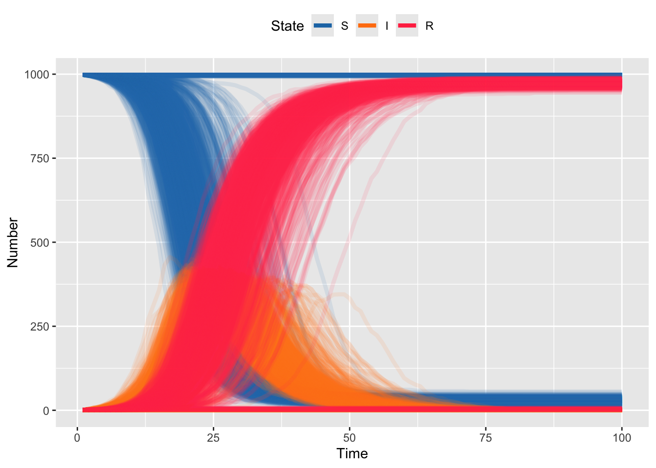
And plotting the simulated trajectories should look pretty close to what we got with Gillespie. But, because we can simulate many more iterations, we can start to observe some of the rarer behavior; e.g. even for simulations with \(R_0 = 3.5\) there are some simulation runs for which the epidemic doesn’t take off (S stays at 1000).
Note that because we have stored the newly infected individuals as “new cases” then we can plot both the incidence (new cases) and prevalence (I) each day.
Code
####################################################################
# plotting                                                         #
####################################################################
# put output in a data frame
tau_df <- tibble(
  S = array(s_mat),
  I = array(i_mat),
  R = array(r_mat),
  N = array(n_mat),
  cases = array(new_cases),
  time = rep(1:max_time, sims),
  iteration = rep(1:sims, each = max_time)
)

tau_df <- tau_df %>%
  pivot_longer(
    # Don't pivot the time column
    cols = -c(time, iteration),
    names_to = "state",
    values_to = "number"
  ) %>%
  mutate(state = factor(state, levels = c("S", "I", "R", "N", "cases")))

# fix this color
sir_colors <- c(S = "#1f77b4", I = "#ff7f0e", R = "#FF3851", cases = "#2ca02c")

tau_df %>%
  mutate(iteration = as.factor(iteration)) %>%
  filter(state %in% c("I", "cases")) %>%
  ggplot(aes(
    x = time,
    y = number,
    group = interaction(iteration, state),
    color = state
  )) +
  geom_line(linewidth = 1.5, alpha = .1) +
  scale_color_manual(values = sir_colors) +
  labs(
    x = "Time",
    y = "Number",
    color = "State"
  ) +
  guides(color = guide_legend(override.aes = list(alpha = 1))) +
  theme(legend.position = "top")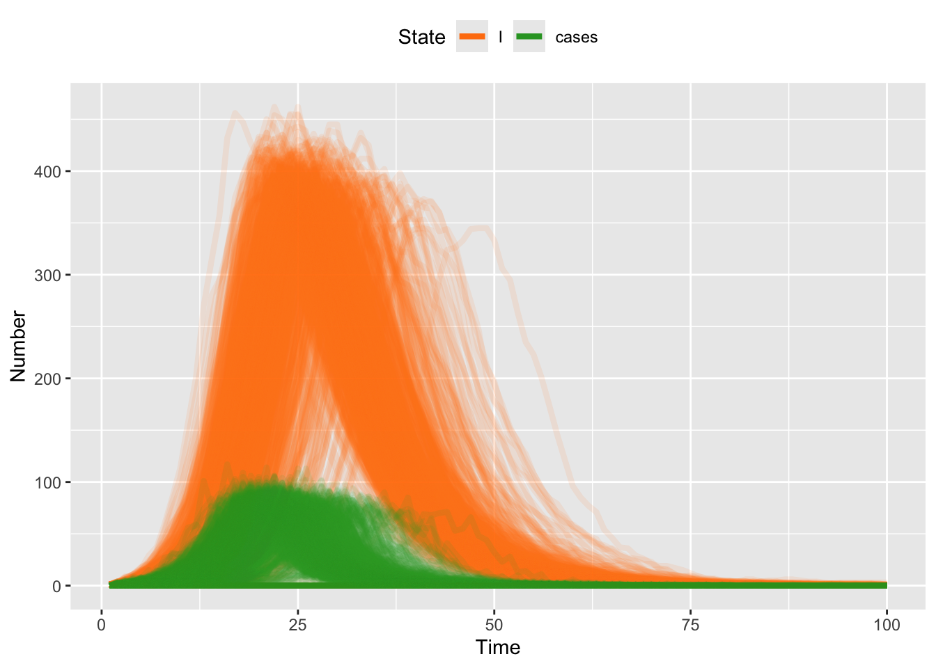
Recall that the time series of new incident cases is very different than the time series of prevalent cases. Recall from our earlier discussion that the former are more likely to be what we would see in clinical surveillance. The latter are what we might see if we did random testing in the population. Which one would you expect to correspond best to environmental wastewater surveillance?
10.5 The Chain Binomial Algorithm
In the last section, we saw that by moving from continuous time to discrete time steps, we limit the complexity (the number of stochastic evaluations scales with time and the number of states, instead of population size and the number of states). You may have also noticed that the individual steps in the Tau Leaping algorithm can be modeled as Poisson or Binomial random variables. Combining these two gives us another common algorithm for stochastic simulation, the Chain Binomial model. Here, we simplify further and use a time step that is equal to the infectious generation period; e.g. 2 weeks for measles, or 1 week for flu. If we assume that time progresses in discrete, non-overlapping generations, then those that get infected at the start of one time step, recover at the end of that time step. This simplification means that we only have to model the infection process as stochastic, and the recovery process at the end of the time step is now deterministic. This is obviously unrealistic, but makes the model much simpler for formal statistical model fitting using likelihood and Bayesian methods. So while it is imperfect, it remains as a common method for “first-pass” analyses.
As before, we start with initial conditions. Here we initialize with the same population as before, but notice that the transmission rate, \(\beta\) is different. Time is rescaled here to units of epidemic generation time, so \(\beta\) is scaled correspondingly and now, for this formulation, \(\beta\) is \(R_0\).
Recall that the basic reproduction number, \(R_0\) is a function of the pathogen and the population of interest. In models, both the population (e.g. mixing, heterogeneity, etc) and the pathogen (e.g. time-scale of recovery) are represented using approximations to the biology. Here, the choice of model forces a change in time-scale which means that we have to change \(\beta\) accordingly; thus, \(\beta\), which is ostensibly a biological parameter is also a property of the model.
Code
####################################################################
# Parameters and initial conditions                                #
####################################################################
S <- 998 # number susceptible
I <- 1 # number infected
R <- 1 # number recovered
time <- 0

beta <- 3.5 # transmission rate -- note the change in value
When we implement the forward simulation, we now only have to generate random draws for the infection process, which again simplifies the amount of stochastic simulation we have to do, and speeds up run times. While this might not be limiting in the scale of this activity, this DOES become an issue when we have to fit stochastic models. Recall from the lecture on parameter estimation that the basic recipe has us build a model and test out all, or many, values of the parameters (here \(\beta\)) to find which one is closest to the data. Here, because each run of the stochastic simulation is different, we need to run simulations over many possible parameters, and for each parameter, we need to run many stochastic runs to characterize the average, or most likely, behavior. So, the number of simulations can rapidly increase into the millions (bigger for models with more parameters), so every bit of savings in computational time can be valuable.
Code
####################################################################
# Single time step                                                 #
####################################################################
chain_binomial_step <- function(sims, S, I, R, beta, ...) {
  # S = initial susceptible population
  # I = initial infected population
  # R = initial recovered population
  # beta is transmission rate

  # total population size
  N <- S + I + R
  # this is the only stochastic step; only do draw if I >0
  new_i <- rbinom(n = sims, pmax(S, 0), 1 - exp(-beta * pmax(I, 0) / N))
  # this step is now deterministic, because everyone from the past time
  # step recovers
  new_s <- S - new_i
  new_r <- R + I

  cbind(new_s, new_i, new_r)
}
Then we can run the simulation over a set of discrete time steps, T. Note again that T is now the number of infectious generation times, since time is rescaled relative to the models above.
Code
####################################################################
# Run over many steps #
####################################################################
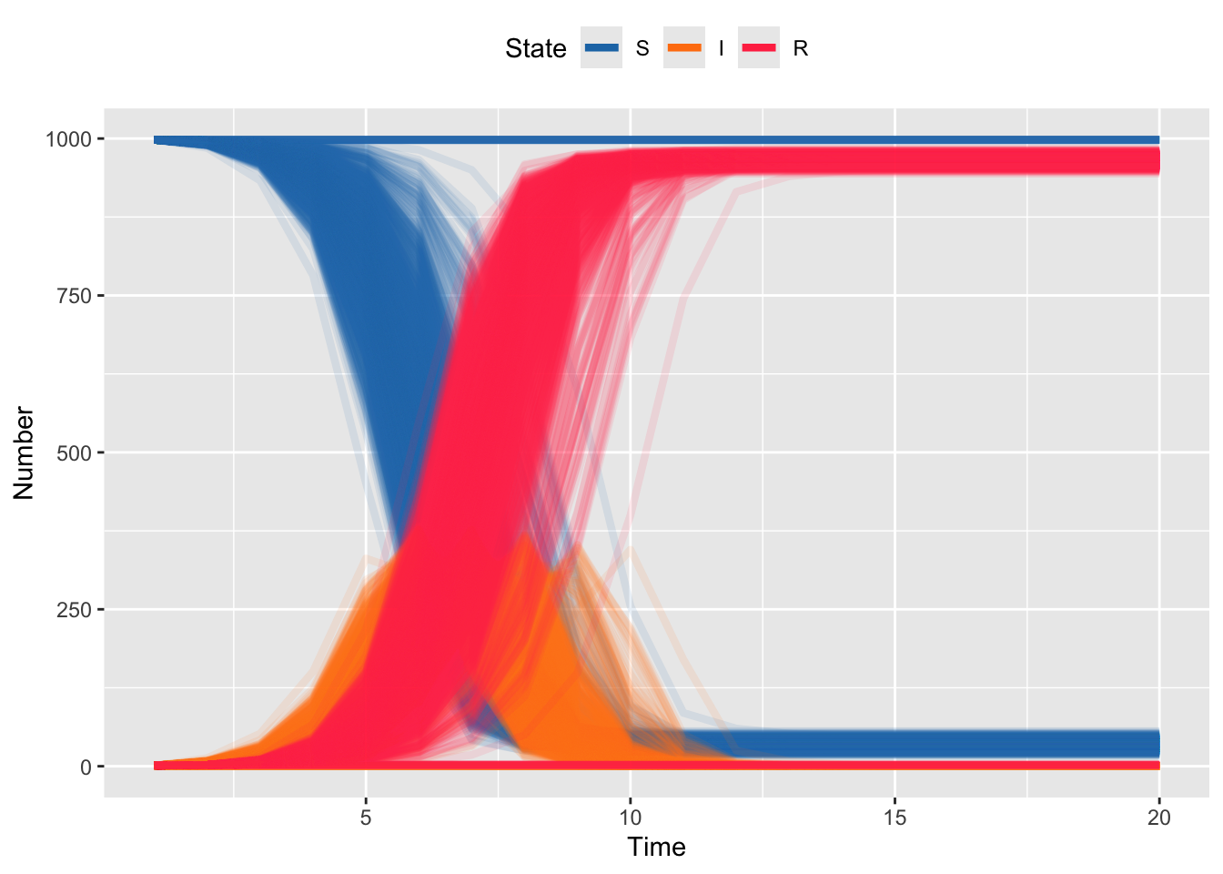
max_time <- 20
# note here that the time step is one infectious generation time,
# so 7 days from gamma above
sims <- 1000
s_mat <- matrix(S, 1, sims) # storage item for S for all simulations
i_mat <- matrix(I, 1, sims) # storage item for I for all simulations
r_mat <- matrix(R, 1, sims) # storage item for R for all simulations
n_mat <- S + I + R
for (time_step in 2:max_time) {
out <- chain_binomial_step(
sims,
s_mat[time_step - 1, ],
i_mat[time_step - 1, ],
r_mat[time_step - 1, ],
beta
)
# update state
s_mat <- rbind(s_mat, out[, 1])
# update state
i_mat <- rbind(i_mat, out[, 2])
# update state
r_mat <- rbind(r_mat, out[, 3])
# update state -- note population size isn't changing, but this could be
# updated with births/deaths
n_mat <- rbind(n_mat, out[, 1] + out[, 2] + out[, 3])
}We can plot, but note again, that this is plotted in terms of epidemic generations on the X-axis, rather than days (as in the previous sections).
Code
# put output in a data frame
bin_df <- tibble(
  S = array(s_mat),
  I = array(i_mat),
  R = array(r_mat),
  N = array(matrix(n_mat)),
  time = rep(1:max_time, sims),
  iteration = rep(1:sims, each = max_time)
)

bin_df <- bin_df %>%
  pivot_longer(
    # Don't pivot the time column
    cols = -c(time, iteration),
    names_to = "state",
    values_to = "number"
  ) %>%
  mutate(state = factor(state, levels = c("S", "I", "R", "N")))

# fix this color
sir_colors <- c(S = "#1f77b4", I = "#ff7f0e", R = "#FF3851")

bin_df %>%
  mutate(iteration = as.factor(iteration)) %>%
  filter(state %in% c("S", "I", "R")) %>%
  ggplot(aes(
    x = time,
    y = number,
    group = interaction(iteration, state),
    color = state
  )) +
  geom_line(linewidth = 1.5, alpha = .1) +
  scale_color_manual(values = sir_colors) +
  labs(
    x = "Time",
    y = "Number",
    color = "State"
  ) +
  guides(color = guide_legend(override.aes = list(alpha = 1))) +
  theme(legend.position = "top")