typeof(1)[1] "double"typeof(1L)[1] "integer"The purpose of this section is to get you up-to-speed with R. If you’re completely unfamiliar with R and RStudio, this should provide you with enough to get started and understand what’s going on in the code (and you can always refer back to this page if you understandably get a little lost), and if you have some experience, then it should provide a sufficient description of the packages and functions that we use in this workshop.
Now you have R set installed and you can access it and are familiar with RStudio, it’s time to learn some of the core features of the language.
We’d strongly recommend you read Hands-On Programming With R by Garett Grolemund and R for DataScience by Hadley Wickham, Mine Çetinkaya-Rundel, and Garrett Grolemund for a deeper understanding of the following concepts (and many more).
An object is anything you can create in R using code, whether that is a table you import from a csv file (that will get converted to a dataframe), or a vector you create within a script. Each object you create has a type. We’ve already mentioned two (dataframes and vectors), but there are plenty more. But before we get into object types, let’s take a step back and look at types in general, thinking about individual elements and the fundamentals.
Generally in programming, we have two broad types of numbers: floating point and integer numbers, i.e., numbers with decimals, and whole numbers, respectively. In R, we have these number types, but a floating point number is called a double. The floating point number is the default type R assigns to number: look at the types assigned when we leave off a decimal place vs. specify type integer by ending a number with an L.
Technically type double is a subset of type numeric, so you will often see people convert numbers to floating points using as.numeric(), rather than as.double(), but the different is semantics. You can confirm this using the command typeof(as.numeric(10)) == typeof(as.double(10))semantics. You can confirm this using the commandtypeof(as.numeric(10)) == typeof(as.double(10))`.
Integer types are not commonly used in R, but there are occasions when you will want to use them e.g., when you need whole numbers of people in a simulation you may want to use integers to enforce this. Integers are also slightly more precise (unless very big or small), so when exactness in whole number is required, you may want to use integers.
R has some idiosyncrasies when it comes to numbers. For the most part, doubles are produced, but occasionally an integer will be produced when you are expecting a double.
For example:
Outside of numbers, we have characters (strings) and boolean types.
A boolean (also known as a logical in R) is a TRUE/FALSE statement. In R, as in many programming languages, TRUE is equal to a value of 1, and FALSE equals 0. There are times when this comes in handy e.g. you need to calculate the number of people that responded to a question, and their responses is coded as TRUE/FALSE, you can just sum the vector of responses (more on vectors shortly).
TRUE == 1[1] TRUEFALSE == 0[1] TRUEA character is anything in quotation marks. This would typically by letter, but is occasionally a number, or other symbol. Other languages make a distinction between characters and strings, but not R.
It is important to note that characters are not parsed i.e., they are not interpreted by R as anything other than a character. This means that despite "1" looking like the number 1, it behaves like a character in R, not a double, so we can’t do addition etc. with it.
"1" + 1Error in "1" + 1: non-numeric argument to binary operatorAs mentioned, anything you can create in R is an object. For example, we can create an character object with the assignment operator (<-).
my_char_obj <- "a"In other languages, = is used for assignment. In R, this is generally avoided to distinguish between creating objects (assignment), and specifying argument values (see the section on functions). However, despite what some purists may say, it really doesn’t matter which one you use, from a practical standpoint.
You will note that when we created our object, it did not return a value (unlike the previous examples, a value was not printed). To retrieve the value of the object (in this case, just print it), we just type out the object name.
my_char_obj[1] "a"In this case, we just create an object with only one element. We can check this using the length() function.
length(my_char_obj)[1] 1We could also create an atomic vector (commonly just called a vector, which we’ll use from here-on in). In fact, my_char_obj is actually an vector, i.e., it is a vector of length 1, as we’ve just seen. Generally, a vector is an object that contains multiple elements that each have the same type.
my_char_vec <- c("a", "b", "c")As we’ll see in the example below, we can give each element in a vector a name, and to highlight that vectors must contain elements of the same type, watch what happens here.
[1] "a" "b" "c" "d"my_named_char_vec a b c d
"a" "b" "c" "1" Because R saw the majority of the first elements in the vector were of type character it coerced the number to a character. This is super important to be aware of, as it can cause errors, particularly when coercion goes in the other direction i.e. trying to create a numeric vector.
All the vector types we’ve mentioned so far map nicely to their corresponding element types. But there is an extension of the character vector used frequently: the factor (and, correspondingly, the ordered vector).
A factor is a vector where there are distinct groups that exist within a vector i.e., they are nominal categorical data. For example, we often include gender as a covariate in epidemiological analysis. There is no intrinsic order, but we would want to account for the groups in the analysis.
An ordered vector is when there is an intrinsic order to the grouping i.e., we have ordinal categorical data. If, for example, we were interested in how the frequency of cigarette smoking is related to an outcome, and we wanted to use binned groups, rather than treating it as a continuous value, we would want to create an ordered vector as the ordering of the different groupings is important.
Let’s use the mtcars dataset (that comes installed with R), and turn the number of cylinders (cyl) into an ordered vector, as there are discrete numbers of cylinders a car engine can have, and the ordering matters. Don’t worry about what $ is doing; we’ll come to that later
my_mtcars <- mtcars
my_mtcars$cyl
[1] 6 6 4 6 8 6 8 4 4 6 6 8 8 8 8 8 8 4 4 4 4 8 8 8 8 4 4 4 8 6 8 4my_mtcars$cyl <- ordered(my_mtcars$cyl)
my_mtcars$cyl [1] 6 6 4 6 8 6 8 4 4 6 6 8 8 8 8 8 8 4 4 4 4 8 8 8 8 4 4 4 8 6 8 4
Levels: 4 < 6 < 8If we wanted to directly specify the ordering of the groups, we can do this using the levels argument i.e.
 [1] 6 6 4 6 8 6 8 4 4 6 6 8 8 8 8 8 8 4 4 4 4 8 8 8 8 4 4 4 8 6 8 4
Levels: 8 < 6 < 4
To create a factor, just replace the ordered() call with factor()
There is another type of vector: the list. Most people do not refer to lists as type of vectors, so we will only refer to them as lists, and atomic vectors will just be referred to as vectors.
Unlike vectors there are no requirements about the form of lists i.e., each element of the list can be completely different. One element could store a vector of numbers, another a model object, another a dataframe, and another a list (i.e. a nested list).
my_list <- list(
    c(1, 2, 3, 4, 5),
    glm(mpg ~ ordered(cyl) + disp + hp, data = mtcars),
    data.frame(column_1 = 1:5, column_2 = 6:10)
)
my_named_list <- list(
    my_vec = c(1, 2, 3, 4, 5),
    my_model = glm(mpg ~ ordered(cyl) + disp + hp, data = my_mtcars),
    my_dataframe = data.frame(column_1 = 1:5, column_2 = 6:10)
)
my_list
[[1]]
[1] 1 2 3 4 5
[[2]]
Call: glm(formula = mpg ~ ordered(cyl) + disp + hp, data = mtcars)
Coefficients:
(Intercept) ordered(cyl).L ordered(cyl).Q disp hp
28.98802 -1.71963 2.31169 -0.02604 -0.02114
Degrees of Freedom: 31 Total (i.e. Null); 27 Residual
Null Deviance: 1126
Residual Deviance: 225.1 AIC: 165.2
[[3]]
column_1 column_2
1 1 6
2 2 7
3 3 8
4 4 9
5 5 10my_named_list$my_vec
[1] 1 2 3 4 5
$my_model
Call: glm(formula = mpg ~ ordered(cyl) + disp + hp, data = my_mtcars)
Coefficients:
(Intercept) ordered(cyl).L ordered(cyl).Q disp hp
28.98802 1.71963 2.31169 -0.02604 -0.02114
Degrees of Freedom: 31 Total (i.e. Null); 27 Residual
Null Deviance: 1126
Residual Deviance: 225.1 AIC: 165.2
$my_dataframe
column_1 column_2
1 1 6
2 2 7
3 3 8
4 4 9
5 5 10Similar to vectors, lists can be named, or unnamed, and also that we they display in slightly different ways: when unnamed, we get the notation [[1]] ... [[3]] to denote the different list elements, and with the named list we get $my_vec ... $my_dataframe. It is often useful to name them, though, as it gives you some useful options when it comes to indexing and extracting values later.
If you’re wondering why we are creating our list elements with the = operator, that’s because we can think of this as an argument in the list() function, where the argument name is the name we want the element to have, and the argument value is the element itself.
Dataframes are the last key object type to learn about. A dataframe is technically a special type of list. Effectively, it is a 2-D table where every column has to have elements of the same type (i.e., is a vector), but the columns can be different types to each other. The other important restriction is that all columns must be the same length, i.e. we have a rectangular dataframe.
As we’ve seen before, we can create a dataframe using this code, where 1:5 is shorthand for a vector that contains the sequence of numbers from 1 to 5, inclusive (i.e., c(1, 2, 3, 4, 5)). We could also write this sequence as seq(1, 5, by = 1), allowing us more control over the steps in the sequence.
my_dataframe <- data.frame(
    column_int = 1:5,
    column_dbl = seq(6, 10, 1),
    column_3 = letters[1:5]
)
Like with every other object type, we can just type in the dataframe’s name to return it’s value, but this tim, let’ explore the structure of the dataframe using the str() function. This function can be used on any of the objects we’ve seen so far, and is particularly helpful when exploring lists. One nice feature of dataframes is that it will explicitly print the columns types.
str(my_dataframe)'data.frame': 5 obs. of 3 variables:
$ column_int: int 1 2 3 4 5
$ column_dbl: num 6 7 8 9 10
$ column_3 : chr "a" "b" "c" "d" ...Matrices are crucial to many scientific fields, including epidemiology, as they are the basis of linear algebra. This course will use matrix multiplication extensively (notably R Session 2), so it is worth knowing how to create matrices.
Much like vectors, all elements in a matrix should be the same type (or they will be coerced if possible, resulting in NA if not). It is unusual to have a non-numeric matrix e.g., a character matrix, but it is possible. When we create our matrix, notice that it fills column-first, much like how we think of matrices in math (i.e., i then j).
my_matrix <- matrix(1:8, nrow = 2)
my_matrix
[,1] [,2] [,3] [,4]
[1,] 1 3 5 7
[2,] 2 4 6 8We’ve got our objects, but now we want to do stuff with them. Without getting into too much detail about Object-Oriented Programming (e.g., the S3 class system in R), there are three mains ways of indexing in R:
[]
[[]]
$
Which method we use depends on the type of object we have. Handily, [] will work for pretty much everything, and we typically only use use [[]] for lists.
With both [] and [[]], we can use the indices i.e., the numbered position of the specific values/elements we want to extract, but if we have named objects, we can pass the names to the [] in a vector.
# Extract elements 1 through 3 inclusively
my_char_vec[1:3]
[1] "a" "b" "c"# Extract the same elements but using their names in a vector
my_named_char_vec[c("a", "b", "c")] a b c
"a" "b" "c" Notice that when we index the named vector we get both the name and the value returned. Many times this is OK, but if we only wanted the value, then you’d index with [[]], but it is important to note that you can only pass one value to the brackets.
my_named_char_vec[[c("a", "b")]]Error in my_named_char_vec[[c("a", "b")]]: attempt to select more than one element in vectorIndexmy_named_char_vec[["a"]][1] "a"If you’re wondering why go through the hassle, it’s because values can change position in the list when we update inputs, such as csv datafiles, or needing to restructure code to make something else work. If we only index with the numeric indices, we run the risk of a silent error being returned i.e., a value is provided to us, but we don’t know that it’s referring to the wrong thing. Indexing with names mean that the element’s position in the vector doesn’t matter, and if it’s accidentally been removed when we updated code, and error will be explicitly thrown as it won’t be able to find the index.
When it comes to indexing lists and dataframes (remember, dataframes are just special lists, so the same methods are available to us), it is more common to use [[]] and $, though there are obviously occasions when [] is useful. Let’s look at my_named_list first.
my_named_list[1]$my_vec
[1] 1 2 3 4 5my_named_list["my_vec"]$my_vec
[1] 1 2 3 4 5my_named_list[[1]][1] 1 2 3 4 5my_named_list[["my_vec"]][1] 1 2 3 4 5my_named_list$my_vec[1] 1 2 3 4 5In the examples above, notice how both [] methods returned the name of the element as well as the values (as it did before with the named vector). This is important as it means we need to extract the values from what is returned before we can do any further indexing i.e., to get the value 3 from the list element my_vec.
We can do the same with the unnamed list, except the last two methods are not available as we do not have a name to use.
my_list[1][[1]]
[1] 1 2 3 4 5my_list[[1]][1] 1 2 3 4 5Because a dataframe is a type of list where the column headers are the element names, we can use [[]] and $ as with the named list.
my_dataframe[1] column_int
1 1
2 2
3 3
4 4
5 5my_dataframe[[1]][1] 1 2 3 4 5my_dataframe["column_int"] column_int
1 1
2 2
3 3
4 4
5 5my_dataframe$column_int[1] 1 2 3 4 5If we wanted to extract a particular value from a column, we can use the following methods.
# indexes i then j, just like in math
my_dataframe[2, 1]
[1] 2# Extract the second element from the first column
my_dataframe[[1]][2][1] 2# Extract the second element from column_int, using the i, j procedure as before
my_dataframe[2, "column_int"][1] 2# Extract the second element from column_int
my_dataframe$column_int[2][1] 2Up until now, we’ve been getting to grips with the core concepts of objects, and indexing them. But when you’re writing code, you’ll want to do things that are relatively complicated to implement, such as solve a set of differential equations. Fortunately, for many areas of computing (and, indeed, epidemiology and statistics), many others have also struggled with the same issues and some have gone one to document their solutions in a way others can re-use them. This is the basis for packages. Someone has packaged up a set of functions for others to re-use.
We’ve mentioned the word function a number of time so far, and we haven’t defined it, but that’s coming soon. For the moment, let’s just look at how we can find, install, and load packages.
As mentioned previously CRAN is a place where many pieces of R code is documents and stored for others to download and use. Not only are the R programming language executables stored in CRAN, but so are user-defined functions that have been turned into packages.
To find packages, you can go to the CRAN website and search by name, but there are far too many for that to be worthwhile - just Google what you want to do and add “r” to the end of your search query, and you’ll likely find what you’re looking for. Once you’ve found a package you want to download, next you need to install it.
Barring any super-niche packages, you should be able to use the following command(s):
install.packages("package to download")
# Download multiple by passing a vector of package names
install.packages(c("package 1", "package 2"))
If for some reason you get an error message saying the package isn’t available on CRAN, first, check for typos, and if you still get an error, you may need to download it directly from GitHub. Read here for more information about using the pak package to download packages from other sources.
Now you have your packages installed, you just need to load them to get any of their functionality. The easiest way is to place this code at the top of your script.
# Quotations are not required, but can be used
library(package to download)
Most of the time, this is fine, but occasionally you will run in to an issue where a function doesn’t work as expected. Sometimes this is because of what’s called a namespace conflict i.e., you have two functions with the same name loaded, and potentially you’re using the wrong verion.
For example, in base R (i.e, these functions come pre-installed when you set up R), there is a filter() function from the {stats} package (as mentioned, we’ll denote this as stats::filter()). Throughout this workshop, you will see library(tidyverse) at the top of the pages to indicate the tidyverse set of packages are being loaded (this is actually a package that installs a bunch of related and useful packages for us). In dplyr (one of the packages loaded by tidyverse) there is also a function called filter(). Because dplyr was loaded after {stats} was loaded (because {stats} is automatically loaded when R is started), the dplyr::filter() function will take precedence. If we wanted to specifically use the {stats} version, we could write this:
# Set the seed for the document so we get the same random numbers sampled
# each time we run the script (assuming it's run in its entirety from start
# to finish)
set.seed(1234)

# Create a cosine wave with random noise
raw_timeseries <- cos(pi * seq(-2, 2, length.out = 1000)) + rnorm(1000, sd = 0.5)

# Calculate 20 day moving average using stats::filter()
smooth_timeseries <- stats::filter(raw_timeseries, filter = rep(1/20, 20), sides = 1)

# Plot raw data
plot(raw_timeseries, col = "grey80")

# Overlay smoothed data
lines(smooth_timeseries, col = "red", lwd = 2)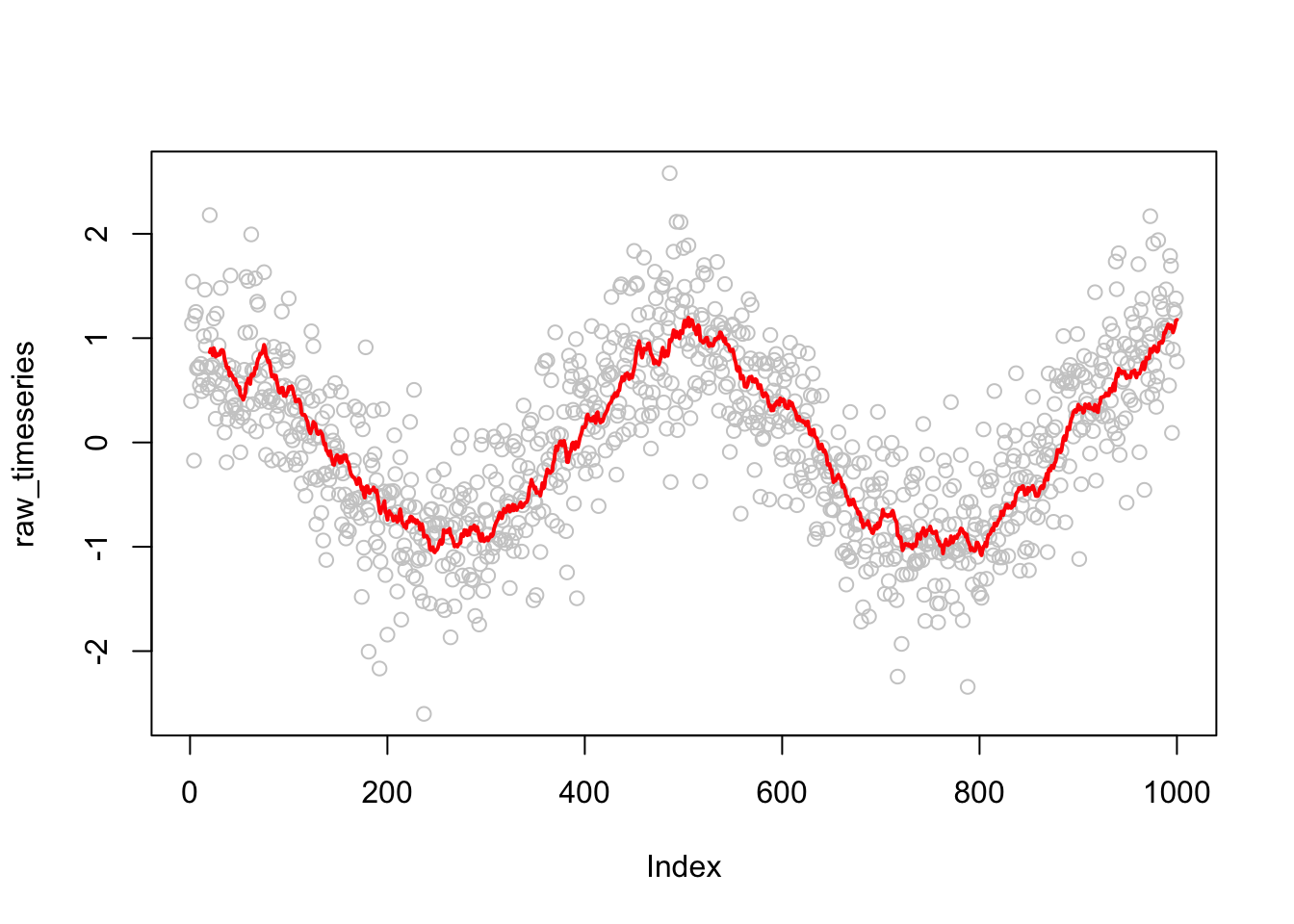
As we’ve alluded to, functions are core to gaining functionality in R. We can always hand-write the code to complete a task, but if we have to repeat a task more than once, it can be tiresome to repeat the same code, particularly if it is a particularly complex task that requires many lines of code. This is where functions come in: they provide us with a mechanism to wrap up code into something that can be re-used. Not only does this reduce the amount of code we need to write, but by minimize code duplication, debugging becomes a lot easier as we only need to remember to make changes and correct one section of our codebase. Say, for example, you want to take a vector of numbers and calculate the cumulative sum e.g.;
my_dbl_vec <- 1:10

cumulative_sum <- 0

for(i in seq_along(my_dbl_vec)) {
    cumulative_sum <- cumulative_sum + i
}

cumulative_sum
[1] 55This is OK if we only do this calculation once, but it’s easy to imagine us wanting to repeat this calculation; for example, we might use calculate the cumulative sum of daily cases to get a weekly incidence over every week of a year. In this situation, we would want to create a function.
my_cumsum <- function(vector) {
    cumulative_sum <- 0

    for(i in seq_along(my_dbl_vec)) {
        cumulative_sum <- cumulative_sum + i
    }

    cumulative_sum
}

my_cumsum(my_dbl_vec)
[1] 55This is obviously a contrived example because, as with many basic operations in R, there is already a function written to perform this calculation that does it in a much more performant and safer manner: cumsum()
For many of the manipulations we will want to perform, a function has already been written by someone else and put into a package that we can download, as we’ve already seen.
There is a special class of functions called anonymous functions that are worth being aware of, as we will use them quite extensively throughout this workshop. As the name might suggest, anonymous functions are functions that are not named, and therefore, not saved for re-use. You may, understandably, be wondering why we would want to use them, given we just make the case for functions replacing repeatable blocks of code. In some instances, we want to be able to perform multiple computations that require creating intermediate objects, but because we only need to use them once, we don’t save them save to our environment, potentially causing issues with conflicts (e.g., accidentally using an object we didn’t mean to, or overwriting existing ones by re-using the same object name). This gets into the broader concept of local vs global scopes, but that is too far beyond the scope of this workshop: see Hands-On Programming with R and Advanced R for more information. Let’s look at an example to see when we might want to use an anonymous function.
Throughout this workshop, we will make use of the map_*() series of functions from the purrr package. We’ll go into more detail about purr::map() shortly, but for now, imagine we have a vector of numbers, and we want to add 5 to each value before and multiplying by 10. The map_dbl() function takes a vector and a function, and outputs a double vector. We could write a function to perform this multiplication, but if we’re only going to do this operation once, it seems unnecessary.
purrr::map_dbl(
    .x = my_dbl_vec,
    .f = function(.x) {
        add_five_val <- .x + 5

        add_five_val * 10
    }
)
[1] 60 70 80 90 100 110 120 130 140 150# only exists within the function
add_five_valError: object 'add_five_val' not foundHere, we’ve specified the anonymous function to take the input .x and multiple each value by 10, and we did it without saving the function. This would be equivalent to writing this:
add_five_multiply_ten <- function(x) {
    add_five_val <- x + 5
    add_five_val * 10
}

purrr::map_dbl(
    .x = my_dbl_vec,
    .f = ~add_five_multiply_ten(.x)
)
[1] 60 70 80 90 100 110 120 130 140 150# only exists within the function
add_five_valError: object 'add_five_val' not foundNotice the ~ used: this specifies that we want to pass arguments into our named function. Without it, we will get an error about .x not being found.
In this example, because we are doing standard arithmetic, R will vectorize our function so that it can automatically be applied to each element of the object, so this example was merely to illustrate the point.
add_five_multiply_ten(my_dbl_vec) [1] 60 70 80 90 100 110 120 130 140 150Before we look at the common packages and functions we use throughout this workshop, let’s take a second to talk about how our data is structured. For much of what we do, it is convenient to work with dataframes, and many functions we will use are designed to work with long dataframes. What this means is that each column represents a variable, and each row is a unique observation.
Let’s first look at a wide dataframe to see how data may be represented. Here, we have one column representing a number for each of the states in the US, and then we have two columns representing some random incidence: one for July and one for August.
wide_df <- data.frame(
    state_id = 1:52,
    july_inc = rbinom(52, 1000, 0.4),
    aug_inc = rbinom(52, 1000, 0.6)
)

wide_df
state_id july_inc aug_inc
1 1 399 613
2 2 409 578
3 3 381 604
4 4 381 607
5 5 387 603
6 6 372 614
7 7 403 597
8 8 407 605
9 9 388 604
10 10 422 595
11 11 343 597
12 12 377 590
13 13 406 618
14 14 421 598
15 15 407 603
16 16 400 614
17 17 387 585
18 18 407 598
19 19 387 604
20 20 405 618
21 21 378 599
22 22 390 601
23 23 399 587
24 24 398 609
25 25 398 591
26 26 401 607
27 27 387 591
28 28 410 603
29 29 396 585
30 30 375 601
31 31 398 596
32 32 406 579
33 33 405 633
34 34 422 607
35 35 395 578
36 36 391 597
37 37 384 568
38 38 426 590
39 39 390 587
40 40 399 586
41 41 373 589
42 42 441 602
43 43 365 600
44 44 397 591
45 45 417 615
46 46 374 606
47 47 398 617
48 48 390 594
49 49 404 579
50 50 403 603
51 51 414 609
52 52 417 606Instead, we reshape this into a long dataframe so that there is a column for the state ID, a column for the month, and a column for the incidence (that is associated with both the state and the month). Using the tidyr package, we could reshape this wide dataframe to be a long dataframe (see this section for more information about the pivot_*() functions)
long_df <- tidyr::pivot_longer(
    wide_df,
    cols = c(july_inc, aug_inc),
    names_to = "month",
    values_to = "incidence",
    # Extract only the month using regex
    names_pattern = "(.*)_inc"
)

long_df
# A tibble: 104 × 3
state_id month incidence
<int> <chr> <int>
1 1 july 399
2 1 aug 613
3 2 july 409
4 2 aug 578
5 3 july 381
6 3 aug 604
7 4 july 381
8 4 aug 607
9 5 july 387
10 5 aug 603
# ℹ 94 more rowsYou will notice that our new dataframe contains three columns still, but is longer than previously; two time as long, in fact.
Particularly keen-eyed reader may also notice that long_df is also has class tibble, not a data.frame. A tibble effectively is a data.frame, but is an object commonly used and output by tidyverse functions, as it has a few extra safety features over the base data.frame.
We’re finally ready to talk about the functions that are used throughout this workshop. The first package to mention is the tidyverse package, which actually a collection of packages: the core packages can be found here. The reason why are using the tidyverse packages throughout this workshop is that they are relatively easily to learn, compared to base R and data.table (not that they are mutually exclusive), and what most people are familiar with. They also are well designed and powerful, so you should be able to do most things you need using their packages.
You can find a list of cheatsheets for all of these packages (and more) here.
Let’s load the tidyverse packages and then go through the key functions used. Unless stated explicitly, these packages will be available to you after loading the tidyverse with the following command.
── Attaching core tidyverse packages ──────────────────────── tidyverse 2.0.0 ──
✔ dplyr     1.1.4     ✔ readr     2.1.5
✔ forcats   1.0.0     ✔ stringr   1.5.1
✔ ggplot2   3.5.2     ✔ tibble    3.3.0
✔ lubridate 1.9.4     ✔ tidyr     1.3.1
✔ purrr     1.0.4
── Conflicts ────────────────────────────────────────── tidyverse_conflicts() ──
✖ dplyr::filter() masks stats::filter()
✖ dplyr::lag()    masks stats::lag()
ℹ Use the conflicted package (<http://conflicted.r-lib.org/>) to force all conflicts to become errorstibble()The tibble is a modern reincarnation of the dataframes that is slightly safer i.e., is more restricted in what you can do with it, and will throw errrors more frequently, but very rarely for anything other than a bug. We will use the terms interchangeably, as most people will just talk about dataframes, as for the most part, they can be treated identically. Use the same syntax as the data.frame() function to create the tibble.
dplyr::filter()If we wanted to take a subset of rows of a dataframe, we would use the dplyr::filter() function. Here, we’re listing the package it’s coming from, as there are some other packages that also export their own version of the filter() function. However, for all the code in this workshop, there aren’t any concerns about namespace conflicts, so we won’t use it from here on in.
The filter() function is relatively simple to work with: you specify the dataframe variable you want to subset by, the filtering criteria, and that’s it. If we include multiple arguments, they get treated as AND statements (&), so all conditions need to be met.
filter(
    long_df,
    month == "july",
    incidence > 410
    # equivalent to: month == "july" & incidence > 410
)
# A tibble: 8 × 3
state_id month incidence
<int> <chr> <int>
1 10 july 422
2 14 july 421
3 34 july 422
4 38 july 426
5 42 july 441
6 45 july 417
7 51 july 414
8 52 july 417We can filter using OR statements (|), so if either condition returns TRUE, then it will be included in the subset.
filter(
    long_df,
    month == "july" | incidence > 600
)
# A tibble: 78 × 3
state_id month incidence
<int> <chr> <int>
1 1 july 399
2 1 aug 613
3 2 july 409
4 3 july 381
5 3 aug 604
6 4 july 381
7 4 aug 607
8 5 july 387
9 5 aug 603
10 6 july 372
# ℹ 68 more rowsselect()If, instead, we wanted to subset of columns of a dataframe, we would use the dplyr::select() function.
Let’s say, from our wide incidence data, we only want the state’s ID and their August incidence. We can directly select the columns this way.
select(
    wide_df,
    state_id, aug_inc
)
state_id aug_inc
1 1 613
2 2 578
3 3 604
4 4 607
5 5 603
6 6 614
7 7 597
8 8 605
9 9 604
10 10 595
11 11 597
12 12 590
13 13 618
14 14 598
15 15 603
16 16 614
17 17 585
18 18 598
19 19 604
20 20 618
21 21 599
22 22 601
23 23 587
24 24 609
25 25 591
26 26 607
27 27 591
28 28 603
29 29 585
30 30 601
31 31 596
32 32 579
33 33 633
34 34 607
35 35 578
36 36 597
37 37 568
38 38 590
39 39 587
40 40 586
41 41 589
42 42 602
43 43 600
44 44 591
45 45 615
46 46 606
47 47 617
48 48 594
49 49 579
50 50 603
51 51 609
52 52 606But in this case, it would be more efficient (for us) to tell R the columns we don’t want. We can do that using the - sign.
select(
    wide_df,
    -july_inc
)
state_id aug_inc
1 1 613
2 2 578
3 3 604
4 4 607
5 5 603
6 6 614
7 7 597
8 8 605
9 9 604
10 10 595
11 11 597
12 12 590
13 13 618
14 14 598
15 15 603
16 16 614
17 17 585
18 18 598
19 19 604
20 20 618
21 21 599
22 22 601
23 23 587
24 24 609
25 25 591
26 26 607
27 27 591
28 28 603
29 29 585
30 30 601
31 31 596
32 32 579
33 33 633
34 34 607
35 35 578
36 36 597
37 37 568
38 38 590
39 39 587
40 40 586
41 41 589
42 42 602
43 43 600
44 44 591
45 45 615
46 46 606
47 47 617
48 48 594
49 49 579
50 50 603
51 51 609
52 52 606If there were multiple columns we didn’t want, we would pass them in a vector.
   state_id
1         1
2         2
3         3
4         4
5         5
6         6
7         7
8         8
9         9
10       10
11       11
12       12
13       13
14       14
15       15
16       16
17       17
18       18
19       19
20       20
21       21
22       22
23       23
24       24
25       25
26       26
27       27
28       28
29       29
30       30
31       31
32       32
33       33
34       34
35       35
36       36
37       37
38       38
39       39
40       40
41       41
42       42
43       43
44       44
45       45
46       46
47       47
48       48
49       49
50       50
51       51
52       52
When it comes to selecting columns, the tidyselect package has a few very handy functions for us. To understand when they are most useful, let’s first look at the mutate() function, and then we’ll highlight how to use the different column selection functions available to use through tidyselect.
mutate()If we have a dataframe and want to add or edit a column, we use the mutate() function. Usually the mutate() function is used to add a column that is related to the existing data, but it is not necessary. Below are examples of both.
# add September incidence that is based on August incidence
mutate(
    wide_df,
    sep_inc = round(aug_inc * 1.2 + rnorm(52, 0, 10), digits = 0)
)
state_id july_inc aug_inc sep_inc
1 1 399 613 735
2 2 409 578 692
3 3 381 604 725
4 4 381 607 733
5 5 387 603 733
6 6 372 614 740
7 7 403 597 726
8 8 407 605 737
9 9 388 604 695
10 10 422 595 710
11 11 343 597 722
12 12 377 590 697
13 13 406 618 732
14 14 421 598 720
15 15 407 603 719
16 16 400 614 719
17 17 387 585 711
18 18 407 598 709
19 19 387 604 729
20 20 405 618 746
21 21 378 599 734
22 22 390 601 723
23 23 399 587 711
24 24 398 609 742
25 25 398 591 705
26 26 401 607 712
27 27 387 591 711
28 28 410 603 737
29 29 396 585 688
30 30 375 601 731
31 31 398 596 715
32 32 406 579 696
33 33 405 633 756
34 34 422 607 739
35 35 395 578 708
36 36 391 597 732
37 37 384 568 672
38 38 426 590 716
39 39 390 587 701
40 40 399 586 693
41 41 373 589 711
42 42 441 602 722
43 43 365 600 728
44 44 397 591 727
45 45 417 615 748
46 46 374 606 720
47 47 398 617 742
48 48 390 594 727
49 49 404 579 707
50 50 403 603 708
51 51 414 609 740
52 52 417 606 724 state_id july_inc aug_inc sep_inc
1 1 399 613 702
2 2 409 578 722
3 3 381 604 711
4 4 381 607 709
5 5 387 603 684
6 6 372 614 682
7 7 403 597 689
8 8 407 605 706
9 9 388 604 688
10 10 422 595 690
11 11 343 597 688
12 12 377 590 674
13 13 406 618 708
14 14 421 598 711
15 15 407 603 718
16 16 400 614 700
17 17 387 585 706
18 18 407 598 680
19 19 387 604 702
20 20 405 618 705
21 21 378 599 701
22 22 390 601 691
23 23 399 587 704
24 24 398 609 689
25 25 398 591 694
26 26 401 607 708
27 27 387 591 703
28 28 410 603 650
29 29 396 585 706
30 30 375 601 713
31 31 398 596 725
32 32 406 579 704
33 33 405 633 690
34 34 422 607 713
35 35 395 578 721
36 36 391 597 716
37 37 384 568 677
38 38 426 590 703
39 39 390 587 708
40 40 399 586 704
41 41 373 589 719
42 42 441 602 697
43 43 365 600 703
44 44 397 591 716
45 45 417 615 721
46 46 374 606 716
47 47 398 617 679
48 48 390 594 706
49 49 404 579 705
50 50 403 603 688
51 51 414 609 717
52 52 417 606 691If we wanted to update a column, we can do that by specifying the column on both sides of the equals sign.
# Update the August incidence to add random noise
mutate(
    wide_df,
    aug_inc = aug_inc + round(rnorm(52, 0, 10), digits = 0)
)
state_id july_inc aug_inc
1 1 399 609
2 2 409 587
3 3 381 614
4 4 381 616
5 5 387 577
6 6 372 605
7 7 403 606
8 8 407 598
9 9 388 608
10 10 422 597
11 11 343 608
12 12 377 583
13 13 406 617
14 14 421 601
15 15 407 616
16 16 400 612
17 17 387 588
18 18 407 585
19 19 387 610
20 20 405 620
21 21 378 605
22 22 390 597
23 23 399 604
24 24 398 608
25 25 398 592
26 26 401 606
27 27 387 599
28 28 410 595
29 29 396 587
30 30 375 607
31 31 398 584
32 32 406 581
33 33 405 627
34 34 422 621
35 35 395 585
36 36 391 580
37 37 384 577
38 38 426 592
39 39 390 581
40 40 399 582
41 41 373 576
42 42 441 606
43 43 365 584
44 44 397 590
45 45 417 620
46 46 374 607
47 47 398 626
48 48 390 595
49 49 404 602
50 50 403 594
51 51 414 624
52 52 417 590One crucial thing to note is that mutate() applies our function/operation to each row simultaneously, so the new column’s value only depends on the row’s original values (or the vector in the case of the second example that didn’t use the values from the data).
paste0()The paste0() function is useful for manipulating objects and coercing them into string, allowing us to do string interpolation. It comes installed with base R, so there’s nothing to install, and because of the way mutate() works, apply functions to each row simultaneously, we can modify whole columns at once, depending on the row’s original values. It works to squish all the values together, without any separators by default. If you wanted spaces between your words, for example, you can use the paste(..., sep = " ") function, which takes the sep argument.
char_df <- mutate(
    long_df,
    # Notice that text is in commas, and object values being passed to paste0()
    # are unquoted.
    state_id = paste0("state_", state_id)
)

char_df
# A tibble: 104 × 3
state_id month incidence
<chr> <chr> <int>
1 state_1 july 399
2 state_1 aug 613
3 state_2 july 409
4 state_2 aug 578
5 state_3 july 381
6 state_3 aug 604
7 state_4 july 381
8 state_4 aug 607
9 state_5 july 387
10 state_5 aug 603
# ℹ 94 more rowsglue::glue()glue() is a function that comes installed with tidyverse, but is not loaded automatically, so you have to reference it explicitly by either using library(glue) or the :: notation shown below. It serves the same purpose as the base paste0(), but in a slightly different syntax. Instead of using a mix of quotations and unquoted object names, glue() requires everything to be in quotation marks, with any value being passed to the string interpolation being enclosed in { }. It is worth learning glue() as it is used throughout the tidyverse packages, such as in the pivot_wider() function.
# A tibble: 104 × 3
   state_id month incidence
   <glue>   <chr>     <int>
 1 state_1  july        399
 2 state_1  aug         613
 3 state_2  july        409
 4 state_2  aug         578
 5 state_3  july        381
 6 state_3  aug         604
 7 state_4  july        381
 8 state_4  aug         607
 9 state_5  july        387
10 state_5  aug         603
# ℹ 94 more rowsstr_replace_all()If we want to replace characters throughout the whole of a string vector, we can do that with the str_replace_all() function. And because dataframes are made up of individual vectors, we can use this to modify vectors.
mutate(
    char_df,
    # pass in the vector (a column, here), the pattern to remove, and the replacement
    clean_state_id = str_replace_all(state_id, "state_", "")
)
# A tibble: 104 × 4
state_id month incidence clean_state_id
<glue> <chr> <int> <chr>
1 state_1 july 399 1
2 state_1 aug 613 1
3 state_2 july 409 2
4 state_2 aug 578 2
5 state_3 july 381 3
6 state_3 aug 604 3
7 state_4 july 381 4
8 state_4 aug 607 4
9 state_5 july 387 5
10 state_5 aug 603 5
# ℹ 94 more rowsacross()Above, we were only mutating a single column at a time, which is what we often do. But, sometimes we want to apply the exact same transformation to multiple columns. For example, say we wanted to turn our monthly incidence data into the average weekly incidence. We could write out each transformation by hand, but when there are more than two columns, this gets rather tedious and introduces the opportunity for mistakes when copying code (one of our motivations for using functions). The tidyselect::across() function allows us to specify the columns we want to apply the transformation, and the function (can be named or anonymous), and that’s it.
There are a couple of points to understand about the code below:
. preceding the cols, fns, and x
.x value in the function argument~ is required to pass arguments into the function. In this case it is an anonymous function using the map_*() syntax. state_id july_inc aug_inc
1 1 93.10000 143.0333
2 2 95.43333 134.8667
3 3 88.90000 140.9333
4 4 88.90000 141.6333
5 5 90.30000 140.7000
6 6 86.80000 143.2667
7 7 94.03333 139.3000
8 8 94.96667 141.1667
9 9 90.53333 140.9333
10 10 98.46667 138.8333
11 11 80.03333 139.3000
12 12 87.96667 137.6667
13 13 94.73333 144.2000
14 14 98.23333 139.5333
15 15 94.96667 140.7000
16 16 93.33333 143.2667
17 17 90.30000 136.5000
18 18 94.96667 139.5333
19 19 90.30000 140.9333
20 20 94.50000 144.2000
21 21 88.20000 139.7667
22 22 91.00000 140.2333
23 23 93.10000 136.9667
24 24 92.86667 142.1000
25 25 92.86667 137.9000
26 26 93.56667 141.6333
27 27 90.30000 137.9000
28 28 95.66667 140.7000
29 29 92.40000 136.5000
30 30 87.50000 140.2333
31 31 92.86667 139.0667
32 32 94.73333 135.1000
33 33 94.50000 147.7000
34 34 98.46667 141.6333
35 35 92.16667 134.8667
36 36 91.23333 139.3000
37 37 89.60000 132.5333
38 38 99.40000 137.6667
39 39 91.00000 136.9667
40 40 93.10000 136.7333
41 41 87.03333 137.4333
42 42 102.90000 140.4667
43 43 85.16667 140.0000
44 44 92.63333 137.9000
45 45 97.30000 143.5000
46 46 87.26667 141.4000
47 47 92.86667 143.9667
48 48 91.00000 138.6000
49 49 94.26667 135.1000
50 50 94.03333 140.7000
51 51 96.60000 142.1000
52 52 97.30000 141.4000everything()If we wanted to select every column in a dataframe, we would use the everything() function. This may not seem helpful initially, but there are occasions when it’s very useful. For instance, in the previous example we still specified the exact columns we wanted to transform. However, if there were five times as many, we wouldn’t want to do that. Do note that if we replaced this with everything(), we would also mutate() our state_id column, which we probably don’t want to do, so we could combine it with the - selection seen previously.
contains()Another very handy function is the tidyselect::contains() function. This allows us to specify a string that the column names must contain for them to be selected. We could change the above example to look like this:
   state_id  july_inc  aug_inc
1         1  93.10000 143.0333
2         2  95.43333 134.8667
3         3  88.90000 140.9333
4         4  88.90000 141.6333
5         5  90.30000 140.7000
6         6  86.80000 143.2667
7         7  94.03333 139.3000
8         8  94.96667 141.1667
9         9  90.53333 140.9333
10       10  98.46667 138.8333
11       11  80.03333 139.3000
12       12  87.96667 137.6667
13       13  94.73333 144.2000
14       14  98.23333 139.5333
15       15  94.96667 140.7000
16       16  93.33333 143.2667
17       17  90.30000 136.5000
18       18  94.96667 139.5333
19       19  90.30000 140.9333
20       20  94.50000 144.2000
21       21  88.20000 139.7667
22       22  91.00000 140.2333
23       23  93.10000 136.9667
24       24  92.86667 142.1000
25       25  92.86667 137.9000
26       26  93.56667 141.6333
27       27  90.30000 137.9000
28       28  95.66667 140.7000
29       29  92.40000 136.5000
30       30  87.50000 140.2333
31       31  92.86667 139.0667
32       32  94.73333 135.1000
33       33  94.50000 147.7000
34       34  98.46667 141.6333
35       35  92.16667 134.8667
36       36  91.23333 139.3000
37       37  89.60000 132.5333
38       38  99.40000 137.6667
39       39  91.00000 136.9667
40       40  93.10000 136.7333
41       41  87.03333 137.4333
42       42 102.90000 140.4667
43       43  85.16667 140.0000
44       44  92.63333 137.9000
45       45  97.30000 143.5000
46       46  87.26667 141.4000
47       47  92.86667 143.9667
48       48  91.00000 138.6000
49       49  94.26667 135.1000
50       50  94.03333 140.7000
51       51  96.60000 142.1000
52 52 97.30000 141.4000rename_with()If we wanted to rename columns of a dataframe, we can use the rename() function. However, like the previous tidyselect examples, sometimes we want to apply the same renaming scheme (function) to the columns. rename_with() allows us to pass a function to multiple columns at once, achieving what we want with minimal effort, and without needing to use across().
rename_with(
    wide_df,
    .cols = contains("_inc"),
    .fn = ~str_replace_all(.x, "_inc", "_incidence")
)
state_id july_incidence aug_incidence
1 1 399 613
2 2 409 578
3 3 381 604
4 4 381 607
5 5 387 603
6 6 372 614
7 7 403 597
8 8 407 605
9 9 388 604
10 10 422 595
11 11 343 597
12 12 377 590
13 13 406 618
14 14 421 598
15 15 407 603
16 16 400 614
17 17 387 585
18 18 407 598
19 19 387 604
20 20 405 618
21 21 378 599
22 22 390 601
23 23 399 587
24 24 398 609
25 25 398 591
26 26 401 607
27 27 387 591
28 28 410 603
29 29 396 585
30 30 375 601
31 31 398 596
32 32 406 579
33 33 405 633
34 34 422 607
35 35 395 578
36 36 391 597
37 37 384 568
38 38 426 590
39 39 390 587
40 40 399 586
41 41 373 589
42 42 441 602
43 43 365 600
44 44 397 591
45 45 417 615
46 46 374 606
47 47 398 617
48 48 390 594
49 49 404 579
50 50 403 603
51 51 414 609
52 52 417 606Hopefully you are noticing a pattern between the tidyselect-type functions. When you need to apply a function to multiple columns in a dataframe, you will select the columns with the .cols argument, and pass the function to the .fn(s) argument with the ~ symbol indicating you are using the .x to represent the column in the function (yes, there is a touch of ambiguity between .fns and .fn, but the general pattern holds). This will be useful when we look at the map_*() family of functions.
magrittr::%>%The %>% operator is an interesting and very useful function that comes installed (and loaded) with the tidyverse package (technically from the magrittr package from within the tidyverse). It allows us to chain together operations without needing to create intermediate objects. Say for example we have our wide incidence data and want to add data for September before turning it into a long dataframe, we could create and intermediate object before using the pivot_longer() function from before, but we might not want to create another object that we don’t really care about. This is when we would want to use a pipe, as it takes the output of one operation and pipes it into the next one.
mutate(
    wide_df,
    sep_inc = round(aug_inc * 1.2 + rnorm(52, 0, 10), digits = 0)
    ) %>%
    pivot_longer(
        cols = c(july_inc, aug_inc, sep_inc),
        names_to = "month",
        values_to = "incidence",
        names_pattern = "(.*)_inc",
        data = .
    )
# A tibble: 156 × 3
state_id month incidence
<int> <chr> <dbl>
1 1 july 399
2 1 aug 613
3 1 sep 725
4 2 july 409
5 2 aug 578
6 2 sep 685
7 3 july 381
8 3 aug 604
9 3 sep 710
10 4 july 381
# ℹ 146 more rowsBy default, the previous object gets input into the first argument of the next function, but here we’ve shown that you can manipulate the position the object is piped into by specify the argument using the . syntax.
|>In R version 4.1.0, the |> was added as the base pipe operator. It works slightly differently to %>%, and frankly, is less powerful and less common (at the moment), so we won’t use it in this workshop.
group_by()If we have groups in our dataframe and want to apply some function to each group’s data, we can use the group_by() function. For example, if we wanted to calculate the mean and median incidence in our fake data from earlier, but group it by the month.
pivot_*()We’ve already seen the purpose of the pivot_longer() function: taking wide data and reshaping it to be long. There is an equivalent to go from long to wide: pivot_wider(). Occassionally this is useful (though it is less common than creating long data).
pivot_wider(
    long_df,
    names_from = month,
    values_from = incidence,
    names_glue = "{month}_inc"
)
# A tibble: 52 × 3
state_id july_inc aug_inc
<int> <int> <int>
1 1 399 613
2 2 409 578
3 3 381 604
4 4 381 607
5 5 387 603
6 6 372 614
7 7 403 597
8 8 407 605
9 9 388 604
10 10 422 595
# ℹ 42 more rowsHere, the names_glue argument is making use of the glue::glue() function (see above) that is installed with tidyverse, but not loaded automatically for use by the users.
map_*()The map_*() functions come from the purrr package (a core part of the tidyverse), and are incredibly useful. They are relatively complicated, so there isn’t enough space to go into full detail, but here we’ll just outline enough so you can read more and understand what’s going on.
We’ve already seen we can apply functions to each element of a vector (atomic or list vectors). The key points to note are the . preceding the x and f arguments. If we use map() we get a list returned, map_dbl() a double vector, map_char() a character vector, map_dfr() a dataframe etc.
In the example below, we’ll walk through map_dfr() as it’s one of the more confusing variants due to the return requirements.
map_dfr_example <- map_dfr(
    .x = my_dbl_vec,
    .f = function(.x) {
        # Note we don't use , at the end of each line - it's as if we were
        # running the code in the console
        times_ten <- .x * 10
        divide_ten <- .x / 10

        # construct a tibble as normal (requires , between arguments)
        tibble(
            original_val = .x,
            times_ten = times_ten,
            divide_ten = divide_ten
        )
    }
)

map_dfr_example
# A tibble: 10 × 3
original_val times_ten divide_ten
<int> <dbl> <dbl>
1 1 10 0.1
2 2 20 0.2
3 3 30 0.3
4 4 40 0.4
5 5 50 0.5
6 6 60 0.6
7 7 70 0.7
8 8 80 0.8
9 9 90 0.9
10 10 100 1 What’s happening under the hood is that map_dfr() is applying the anonymous function we defined to each element in our vector and returning a list of dataframes that contains one row and three columns, i.e. for the first element, we would get this:
list(map_dfr_example[1, ])[[1]]
# A tibble: 1 × 3
original_val times_ten divide_ten
<int> <dbl> <dbl>
1 1 10 0.1It then calls the bind_rows() function to squash all of those dataframes together, one row stacked on top of the next, to create one large dataframe. We could write the equivalent code like this:
bind_rows(
    map(
    .x = my_dbl_vec,
    .f = function(.x) {
        # Note we don't use , at the end of each line - it's as if we were
        # running the code in the console
        times_ten <- .x * 10
        divide_ten <- .x / 10

        # construct a tibble as normal (requires , between arguments)
        tibble(
            original_val = .x,
            times_ten = times_ten,
            divide_ten = divide_ten
        )
    }
)
)
# A tibble: 10 × 3
original_val times_ten divide_ten
<int> <dbl> <dbl>
1 1 10 0.1
2 2 20 0.2
3 3 30 0.3
4 4 40 0.4
5 5 50 0.5
6 6 60 0.6
7 7 70 0.7
8 8 80 0.8
9 9 90 0.9
10 10 100 1 map_dfc() does exactly the same thing, but calls bind_cols() instead, to place the columns next to each other.
There is one more important variant to go through: pmap_*(). If map_*() takes one vector as an argument, pmap_*() takes a list of arguments. What this means is that we can iterate through the elements of as many arguments as we’d like, in sequence. For example, let’s multiply the elements of two double vectors together.
# Create a second vector of numbers
my_second_dbl_vec <- rnorm(length(my_dbl_vec), 20, 20)
my_second_dbl_vec
[1] 45.583594 7.463083 20.505265 46.030180 15.004206 22.699967 17.066535
[8] 44.678612 22.708520 21.344806# Remind ourselves what our original vector looks like
my_dbl_vec [1] 1 2 3 4 5 6 7 8 9 10pmap_dbl(
.l = list(first_num = my_dbl_vec, sec_num = my_second_dbl_vec),
.f = function(first_num, sec_num) {
first_num * sec_num
}
) [1] 45.58359 14.92617 61.51580 184.12072 75.02103 136.19980 119.46575
[8] 357.42890 204.37668 213.44806There are a couple of important points to note here:
.l instead of .x to denote we are passing a list() of vectors.list(), which are then used within the function itself (similar to how we used .x in our map_*() functions)As before, this is an unnecessary approach as R would vectorize the operation, but it is useful to demonstrate the principle.
my_dbl_vec * my_second_dbl_vec [1] 45.58359 14.92617 61.51580 184.12072 75.02103 136.19980 119.46575
[8] 357.42890 204.37668 213.44806nest()Nesting is a relatively complex, but powerful, concept, particularly when combined with the map_*() functions. Commonly, as in this workshop, it is used to apply a model function to multiple different datasets, and store them all in one dataframe for easy of manipulation. What it effectively does is group your existing dataframe by a variable, and then shrink all the columns (except the grouping column), into a single list column, leaving you with as many rows as there are distinct groups. Each element of the new list column is itself a small dataframe that contains all the original variables and data, but only those that are relevant for the group. Hopefully this example will make it clearer. Here, we’ll take the mtcars dataset, and like before, we’ll group by the cyl variable, but this time we’ll nest the rest of the data.
nested_mtcars <- nest(mtcars, data = -cyl)
nested_mtcars
# A tibble: 3 × 2
cyl data
<dbl> <list>
1 6 <tibble [7 × 10]>
2 4 <tibble [11 × 10]>
3 8 <tibble [14 × 10]>We can see we’ve nested all columns, except cyl. Looking at the data column for just the first row (cyl == 6), we see we have a list with one item: the rest of the data that’s relevant to the rows where cyl == 6 (notice the [[1]] above the tibble).
nested_mtcars[1, ]$data[[1]]
# A tibble: 7 × 10
mpg disp hp drat wt qsec vs am gear carb
<dbl> <dbl> <dbl> <dbl> <dbl> <dbl> <dbl> <dbl> <dbl> <dbl>
1 21 160 110 3.9 2.62 16.5 0 1 4 4
2 21 160 110 3.9 2.88 17.0 0 1 4 4
3 21.4 258 110 3.08 3.22 19.4 1 0 3 1
4 18.1 225 105 2.76 3.46 20.2 1 0 3 1
5 19.2 168. 123 3.92 3.44 18.3 1 0 4 4
6 17.8 168. 123 3.92 3.44 18.9 1 0 4 4
7 19.7 145 175 3.62 2.77 15.5 0 1 5 6Now we can use map to fit a model to this subsetted data.
# A tibble: 3 × 3
    cyl data               model_fit
  <dbl> <list>             <list>
1     6 <tibble [7 × 10]>  <glm>
2     4 <tibble [11 × 10]> <glm>
3     8 <tibble [14 × 10]> <glm>
This creates a list column (because we used the map() function, which returns a list) that contains the relevant model fits.
It is important to note that there is also a function called nest_by(). However, it returns a rowwise tibble, i.e., any later manipulations will be applied on a row-by-row basis, unlike a standard tibble that applies the manipulation to every row all at once, so we would need to use normal mutate() syntax (and explicitly return a list column) to get the same effect as before.
ggplot()To create out plots, we can use the base plot() functions, but ggplot2 package provides a clean and consistent interface to plotting that has many benefits. In essence, plots are built up in layers, with each stacking on top of the previous.
To initialize a plot, we simply use the ggplot() function call, that creates the background of a figure. Now we need to add data, and geoms to interpret that data.
Let’s use the mtcars dataset again.
mtcars mpg cyl disp hp drat wt qsec vs am gear carb
Mazda RX4 21.0 6 160.0 110 3.90 2.620 16.46 0 1 4 4
Mazda RX4 Wag 21.0 6 160.0 110 3.90 2.875 17.02 0 1 4 4
Datsun 710 22.8 4 108.0 93 3.85 2.320 18.61 1 1 4 1
Hornet 4 Drive 21.4 6 258.0 110 3.08 3.215 19.44 1 0 3 1
Hornet Sportabout 18.7 8 360.0 175 3.15 3.440 17.02 0 0 3 2
Valiant 18.1 6 225.0 105 2.76 3.460 20.22 1 0 3 1
Duster 360 14.3 8 360.0 245 3.21 3.570 15.84 0 0 3 4
Merc 240D 24.4 4 146.7 62 3.69 3.190 20.00 1 0 4 2
Merc 230 22.8 4 140.8 95 3.92 3.150 22.90 1 0 4 2
Merc 280 19.2 6 167.6 123 3.92 3.440 18.30 1 0 4 4
Merc 280C 17.8 6 167.6 123 3.92 3.440 18.90 1 0 4 4
Merc 450SE 16.4 8 275.8 180 3.07 4.070 17.40 0 0 3 3
Merc 450SL 17.3 8 275.8 180 3.07 3.730 17.60 0 0 3 3
Merc 450SLC 15.2 8 275.8 180 3.07 3.780 18.00 0 0 3 3
Cadillac Fleetwood 10.4 8 472.0 205 2.93 5.250 17.98 0 0 3 4
Lincoln Continental 10.4 8 460.0 215 3.00 5.424 17.82 0 0 3 4
Chrysler Imperial 14.7 8 440.0 230 3.23 5.345 17.42 0 0 3 4
Fiat 128 32.4 4 78.7 66 4.08 2.200 19.47 1 1 4 1
Honda Civic 30.4 4 75.7 52 4.93 1.615 18.52 1 1 4 2
Toyota Corolla 33.9 4 71.1 65 4.22 1.835 19.90 1 1 4 1
Toyota Corona 21.5 4 120.1 97 3.70 2.465 20.01 1 0 3 1
Dodge Challenger 15.5 8 318.0 150 2.76 3.520 16.87 0 0 3 2
AMC Javelin 15.2 8 304.0 150 3.15 3.435 17.30 0 0 3 2
Camaro Z28 13.3 8 350.0 245 3.73 3.840 15.41 0 0 3 4
Pontiac Firebird 19.2 8 400.0 175 3.08 3.845 17.05 0 0 3 2
Fiat X1-9 27.3 4 79.0 66 4.08 1.935 18.90 1 1 4 1
Porsche 914-2 26.0 4 120.3 91 4.43 2.140 16.70 0 1 5 2
Lotus Europa 30.4 4 95.1 113 3.77 1.513 16.90 1 1 5 2
Ford Pantera L 15.8 8 351.0 264 4.22 3.170 14.50 0 1 5 4
Ferrari Dino 19.7 6 145.0 175 3.62 2.770 15.50 0 1 5 6
Maserati Bora 15.0 8 301.0 335 3.54 3.570 14.60 0 1 5 8
Volvo 142E 21.4 4 121.0 109 4.11 2.780 18.60 1 1 4 2Looking at the data, we might be interested in how the mpg of a car is affected by it horsepower (hp). To add data, we just use the ggplot() function argument data = mtcars. We also need to tell ggplot() how to map the data points to the figure, i.e., the values for the x and y axes.
Because this depends on the underlying data, this must go within an argument called aes() i.e., aes(x = hp, y = mpg).
To add a layer to show the data, we add a geom. In this case, because we have continuous independent and dependent variables, we could use the geom_point() geom, that will give us a scatter plot. Much like basic arithmetic, we add layers using the + operator.
ggplot(data = mtcars, aes(x = hp, y = mpg)) +
    geom_point()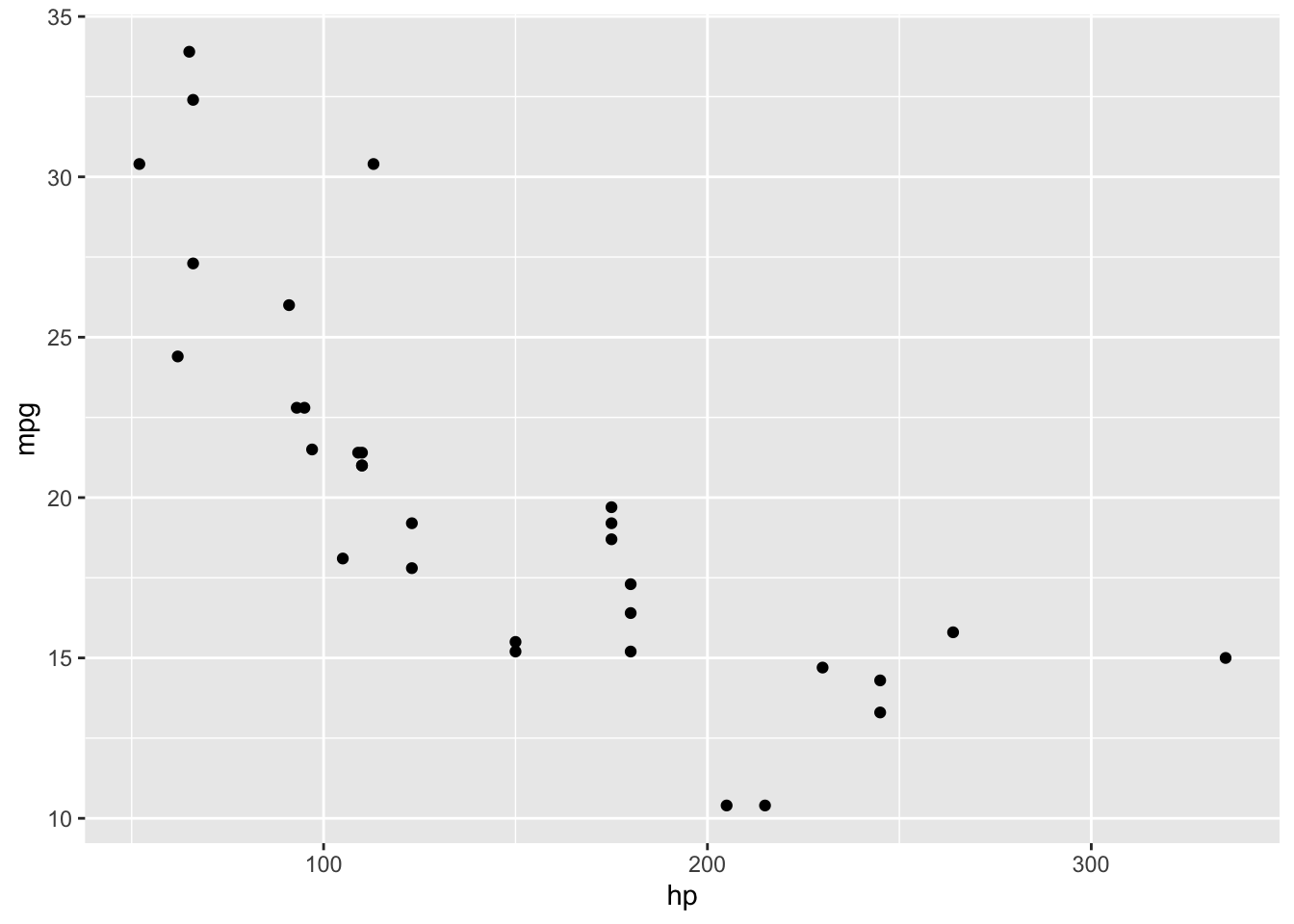
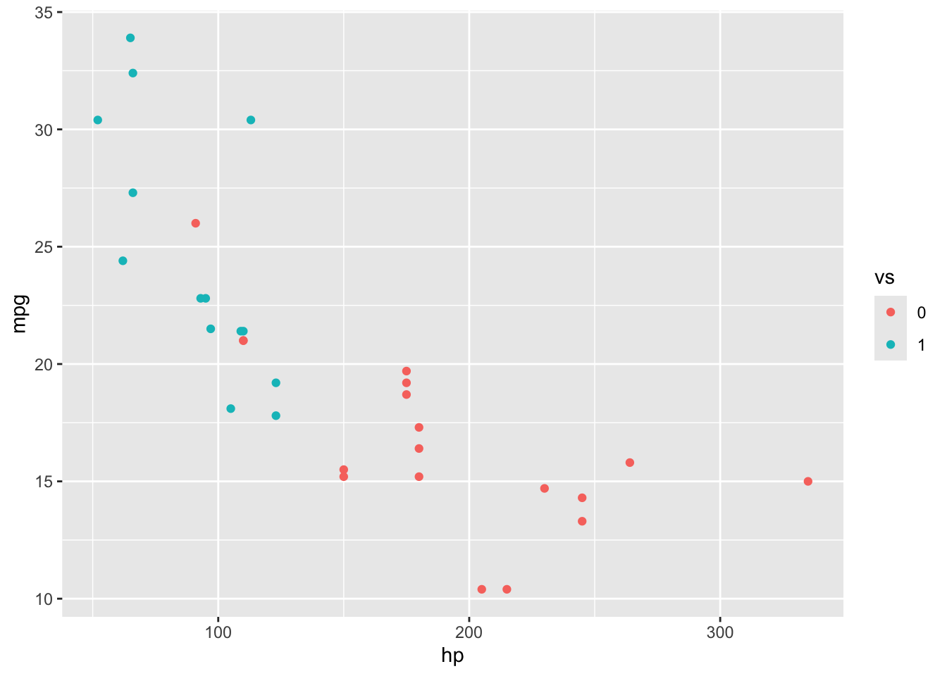
Now let’s imagine we wanted to explore this relationship, but separated by engine type (the vs column). We can use color to separate these points. Because this is an argument that depends on the underlying data, again, this must be placed within aes().
ggplot(data = mtcars, aes(x = hp, y = mpg, color = vs)) +
    geom_point()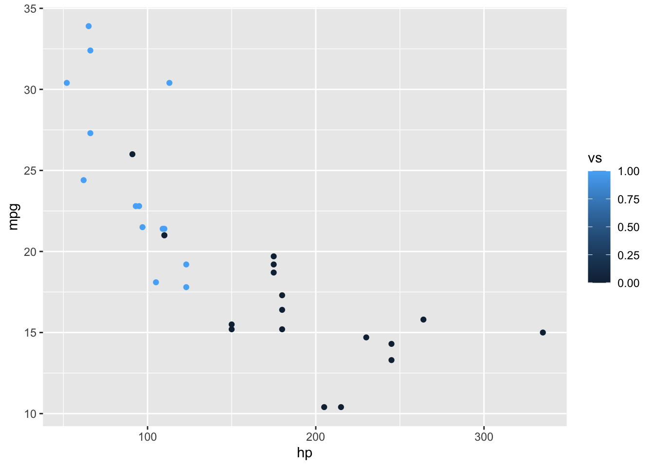
What you’ll notice here is that despite vs being a binary choice, because it is of type double, ggplot() interprets this as a number, so provides a continuous color scale. To correct this, let’s convert vs into a factor before plotting.
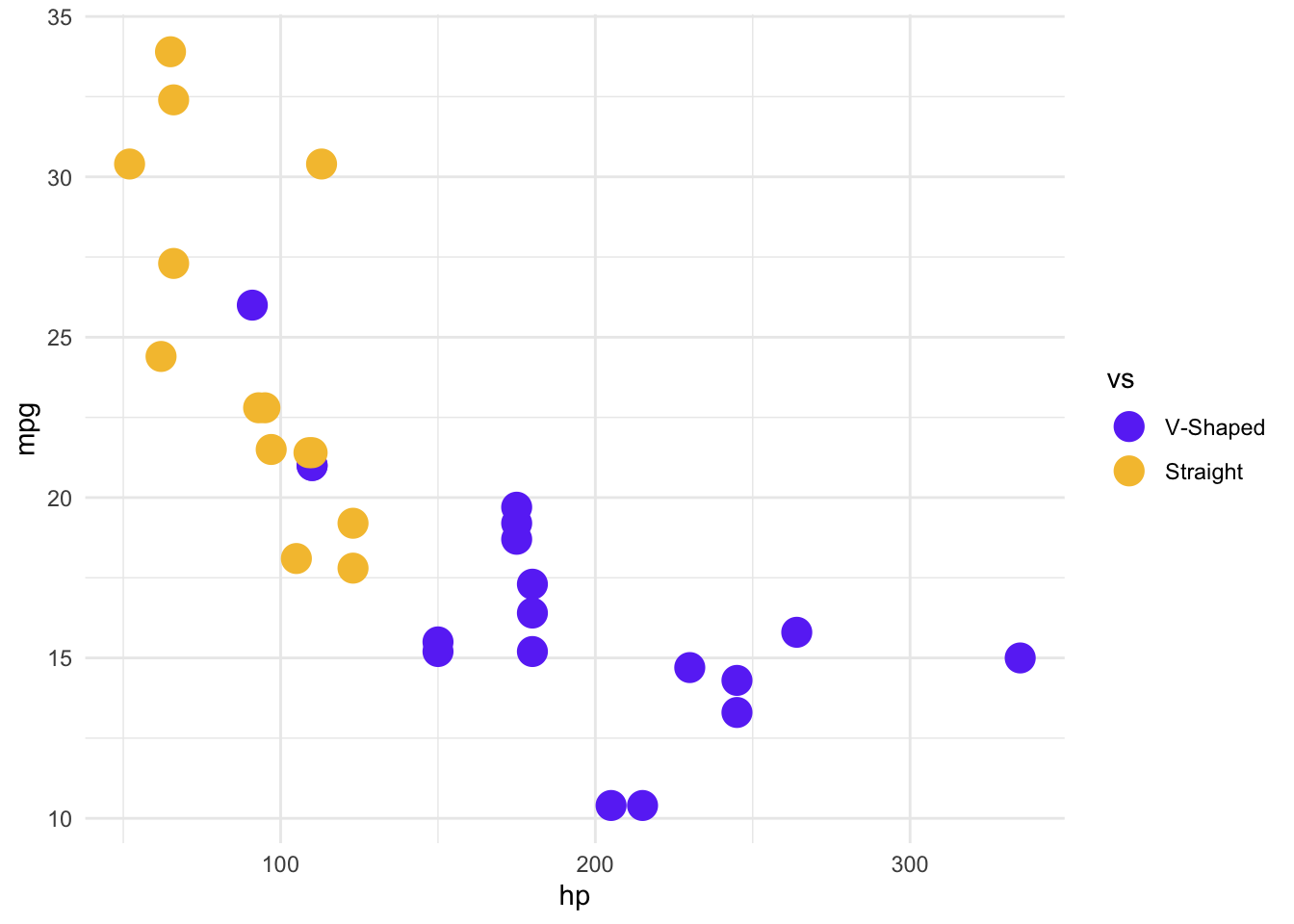
We can change the theme by layering in more information, as we did with the other plotting layers. Here, let’s change the background to white, and add some different colors. We’ll also change the size of the points.
mtcars %>%
    mutate(vs = factor(vs)) %>%
    ggplot(aes(x = hp, y = mpg, color = vs)) +
    geom_point(size = 5) +
    theme_minimal() +
    # We don't need to specify the relationship between the levels and the colors
    # and labels, but it means we're less likely to make a mistake in interpretation
    # and labelling
    scale_color_manual(
        values = c("0" = "#6b3df5ff", "1" = "#f5c13cff"),
        labels = c("0" = "V-Shaped", "1" = "Straight")
    )
Imagine we wanted to use one more grouping: automatic vs manual transmission (am). Rather than adding yet another color, we could do something called a facet_wrap(), which creates separate panels for each group. Adding this to a ggplot() is very easy - it’s just another + operation! As before, we will add labels for easier interpretation.
mtcars %>%
    mutate(vs = factor(vs)) %>%
    ggplot(aes(x = hp, y = mpg, color = vs)) +
    geom_point(size = 5) +
    theme_minimal() +
    # We don't need to specify the relationship between the levels and the colors
    # and labels, but it means we're less likely to make a mistake in interpretation
    # and labelling
    scale_color_manual(
        values = c("0" = "#6b3df5ff", "1" = "#f5c13cff"),
        labels = c("0" = "V-Shaped", "1" = "Straight")
    ) +
    facet_wrap(~am, labeller = as_labeller(c("0" = "Automatic", "1" = "Manual")))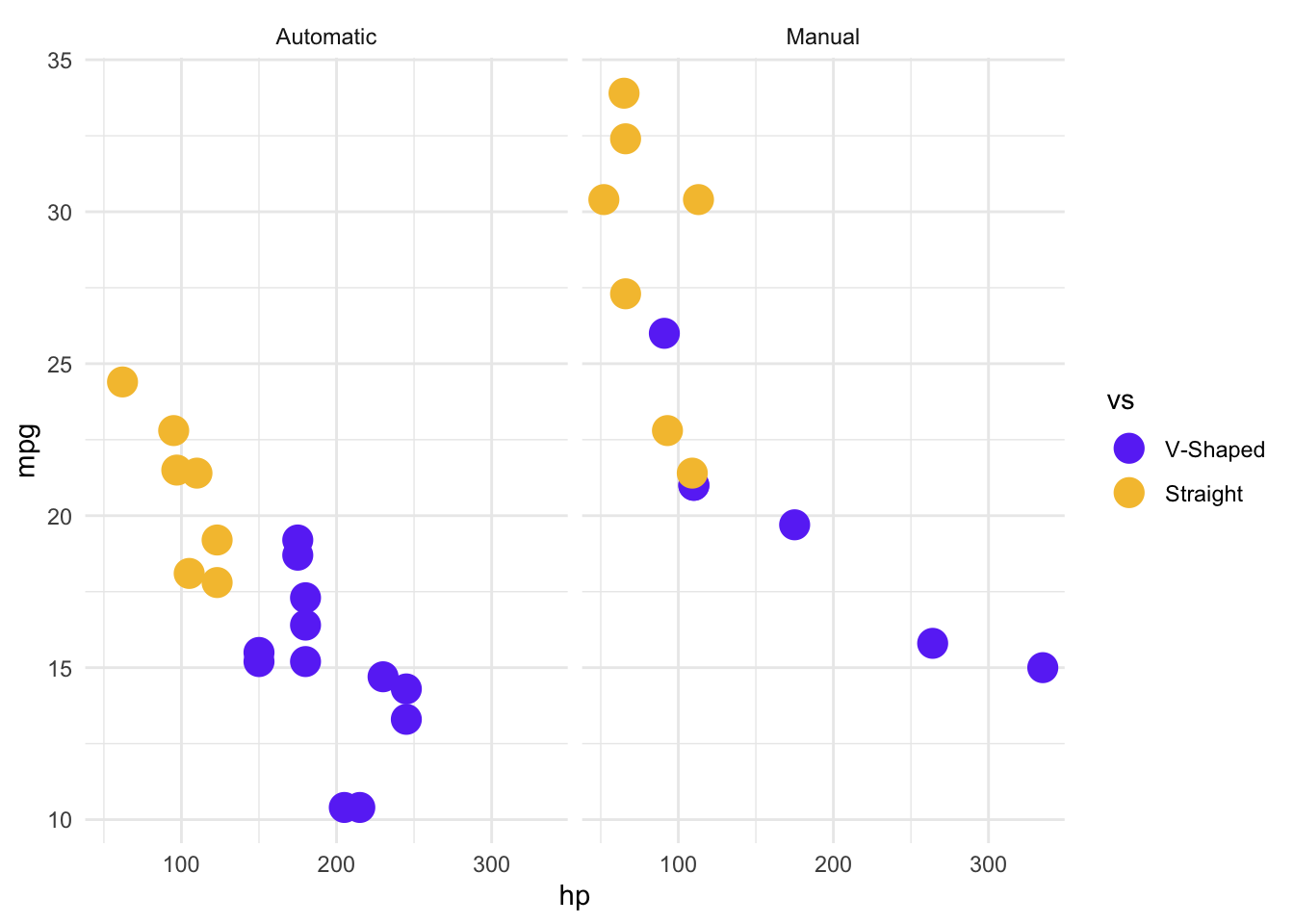
This is looking much better, but we might want to add a line to show the trends within the groups. Again, this is as simple as adding another layer. One thing to note about the plot below, because we specified the data and aes() arguments in the original ggplot() function call, those data relationships will also be applied to our new geom. We could just as easily write them within the geom_*() explicitly, but then we would have to do that for each geom_*() in our plot, which is unnecessary when they all have the same data relationships. To demonstrate this, let’s also make a small modification so that only the points are colored, and the lines are all red. To do that, we will remove color = vs from the global aes(), and add it to one specific to geom_point(). But because we still want to fit a linear model to the different engine types (vs) separately, we will add group = vs to the geom_smooth(aes(), ...) call, to let ggplot() know to treat them as separate groups for the geom_smooth() Because the line color doesn’t depend on the data, it is not in an aes() argument call.
mtcars %>%
    mutate(vs = factor(vs)) %>%
    ggplot(aes(x = hp, y = mpg)) +
    geom_point(aes(color = vs), size = 5) +
    geom_smooth(aes(group = vs), color = "red", method = "lm") +
    theme_minimal() +
    # We don't need to specify the relationship between the levels and the colors
    # and labels, but it means we're less likely to make a mistake in interpretation
    # and labelling
    scale_color_manual(
        values = c("0" = "#6b3df5ff", "1" = "#f5c13cff"),
        labels = c("0" = "V-Shaped", "1" = "Straight")
    ) +
    facet_wrap(~am, labeller = as_labeller(c("0" = "Automatic", "1" = "Manual")))
`geom_smooth()` using formula = 'y ~ x'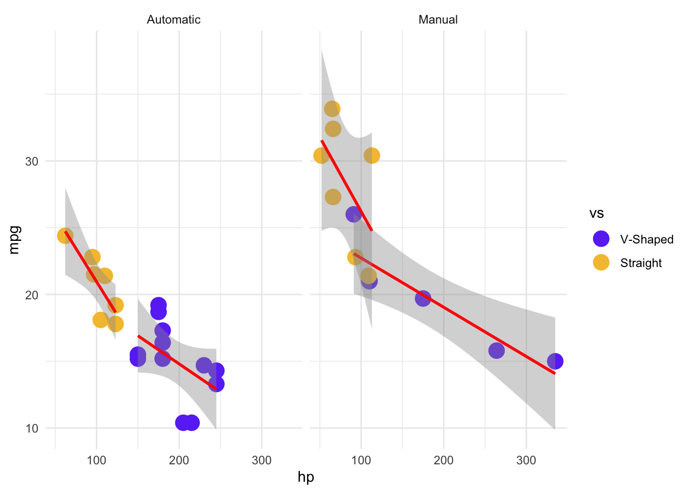
As you can see, once you get used to it, the layering system makes it relatively intuitive to build complex and interesting plots. We’ve only stratched the surface here, so be sure to read the suggested books and the {ggplot2} cheatsheet for more information.
%*%This is the matrix multiplication operator. It works exactly as you’d expect given matrix multiplication rules. As such, you can use it on any combination of vectors and matrices.
As you can see below, R treats vectors as dimensionless, and will try to convert it to either a row or column vector, depending on what makes sense for the matrix multiplication
my_dbl_vec %*% my_second_dbl_vec [,1]
[1,] 1412.086my_matrix <- matrix(1:60, nrow = 10)
my_matrix [,1] [,2] [,3] [,4] [,5] [,6]
[1,] 1 11 21 31 41 51
[2,] 2 12 22 32 42 52
[3,] 3 13 23 33 43 53
[4,] 4 14 24 34 44 54
[5,] 5 15 25 35 45 55
[6,] 6 16 26 36 46 56
[7,] 7 17 27 37 47 57
[8,] 8 18 28 38 48 58
[9,] 9 19 29 39 49 59
[10,] 10 20 30 40 50 60my_dbl_vec [1] 1 2 3 4 5 6 7 8 9 10my_dbl_vec %*% my_matrix [,1] [,2] [,3] [,4] [,5] [,6]
[1,] 385 935 1485 2035 2585 3135my_matrix %*% my_dbl_vecError in my_matrix %*% my_dbl_vec: non-conformable argumentsError in my_matrix %*% t(my_dbl_vec): non-conformable arguments [,1]
[1,] 385
[2,] 935
[3,] 1485
[4,] 2035
[5,] 2585
[6,] 3135